Z and t Statistics for Two Independent Samples

Z AND t STATISTICS FOR TWO INDEPENDENT SAMPLES

Now consider a situation in which we compare the difference between means of samples selected from two populations. In a clinical trial, we could be comparing the mean of a variable (commonly referred to as an endpoint) for a control group to the corresponding mean for a treatment group.

First assume that both groups have normally distributed observations with known and possibly different variances σ_t and σ_c for the treatment and control groups, respectively. Assume that the sample size for the treatment group is n_t and for the control group is n_c. Also assume that the means are μ_t and μ_c for the treatment and control groups, respectively.

Let us select two samples independently from the two groups (treatment and control) and compute the means of the samples. We denote the means of the samples from the control and treatment groups, _t and _c, respectively. The difference between the sample means _t c comes from a normal distribution with mean μ_t – μ_c, variance (σ²_t/n_t) + (σ²_c/n_c), and standard error for t – c equal to √(σ_t /n_t) + (σ_c/n_c). The Z transformation of t – c is defined as

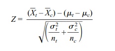
which has a standard normal distribution. Here is an interesting statistical observation: Even though we are finding the difference between two sample means, the variance of the distribution of their differences is equal to the sum of the two squared standard errors associated with each of the individual sample means. The standard errors of the treatment and control groups are calculated by dividing the population variance of each group by the respective sample size of each independently selected sample.

As demonstrated in Section 8.6, the Z transformation, which employs the addition of the error variances of the two means, enables us to obtain confidence intervals for the difference between the means. In the special case where we can assume that σ²_t = σ _c² = σ², the Z formula reduces to

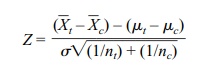
The term σ² is referred to as the common variance. Since P{[–1.96 ≤ Z ≤ 1.96] = 0.95, we find after algebraic manipulation that

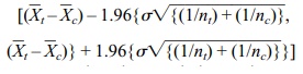
is a 95% confidence interval for μ_t – μ_c.

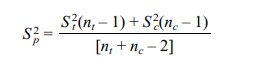
In practice, the population variances of the treatment and control groups are unknown; if the two variances can be assumed to be equal, we can calculate an estimate of the common variance σ², called the pooled estimate. Let S ²_t and S_c² be the sample estimates of the variance for the treatment and control groups, respectively. The pooled variance estimate S_p² is then given by the formula

The corresponding t statistic is

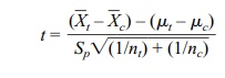
This formula is obtained by replacing the common s in the formula above for Z with the pooled estimate S_p. The resulting statistic has Student’s t distribution with n_t + n_c – 2 degrees of freedom. We will use this formula in Section 8.7 to obtain a confidence interval for the mean difference based on this t statistic when the popu-lation variances can be assumed to be equal.

Although not covered in this text, the hypothesis of equal variances can be tested by an F test similar to the F tests that are used in the analysis of variance (discussed in Chapter 13). If the F test indicates that the variances are different, then one should use a statistic based on the assumption of unequal variances.

This problem with unequal and unknown variances is called the Behrens–Fisher problem. Let “k” denote the test statistic that is commonly used in the Behrens– Fisher problem. The test statistic k does not have a t distribution, but it can be ap-proximated by a t distribution with a degrees of freedom parameter that is not nec-essarily an integer. The statistic k is obtained by replacing the Z statistic in the un-equal variance case as given below:

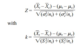
where S²_t and S _c² are the sample estimates of variance for the treatment and control groups, respectively.

We use a t distribution with v degrees of freedom to approximate the distribution of k. The degrees of freedom v are

This is the formula we use for confidence intervals in Section 8.7 when the vari-ances are assumed to be unequal and also for hypothesis testing under the same as-sumptions (not covered in the text).