Wilcoxon Rank-Sum Test

WILCOXON RANK-SUM TEST (THE MANN–WHITNEY TEST)

A nonparametric analog to the unpaired t test, the Wilcoxon rank-sum test is used to compare central tendency, i.e., the locations of two independent samples selected from two populations. Conover (1999) is an important reference for this test. The data must be taken from a continuous scale and represent at least ordinal measure-ment. The Wilcoxon test statistic is calculated by taking the sum of the ranks of n₁ observations from group one. There are also n₂ observations in group two, but only group one is needed to perform the test. The sum of all the ranks (T + T’) is (n₁ + n₂)(n₁ + n₂ + 1)/2. Referring to Table 14.2: (5 + 5)(5 + 5 + 1)/2 = 55. You can veri-fy this sum by checking Table 14.2. Since n₁/(n₁ + n₂) is the probability that a randomly selected observation is from group one, multiplying these two numbers to-gether gives the expected rank sum for group one. This value is (n₁)(n₁ + n₂ + 1)/2 = (5)(11)/2 = 27.5. We will use the rank sum for group one as the test statistic. The distribution of the rank sum can be found in tables for small to moderate values of n₁ and n₂. For n₁ = 5 and n₂ = 5, the critical value is 18. A rank sum that is less than 18 or greater than 55 – 18 = 37 is significant (p < 0.05, two-tailed test). Thus, in our example, since T = 25 the difference between the treatment and control groups is not statistically significant.

Here is a second example that uses small sample sizes. Recall in Section 8.7 the table for pig blood loss data to compare the treatment and the control groups. In Section 9.9, we used these data to demonstrate the two-sample t test when both of the variances for the parent population are assumed to be unknown and equal. Note that if the variances are equal, we are only entertaining the possibility of a differ-ence in the center or median of the distribution. Because these data did not fit well to the normal distribution, we might perform a Wilcoxon rank-sum test to deter-mine whether we can detect differences between the medians of the two popula-tions. Table 14.3 shows the data and the pooled ranks.

TABLE 14.3. Pig Blood Loss Data (ml)

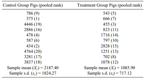
The ranks in Table 14.3 are obtained as follows. First we list all the data irre-spective of control group or treatment group assignment: 786, 375, 4446, 2886, 478, 587, 434, 4764, 3281, 3837, 543, 666, 455, 823, 1716, 797, 2828, 1251, 702, 1078. Next we rearrange these values from smallest to largest: 375, 434, 455, 478, 543, 587, 666, 702, 786, 797, 823, 1078, 1251, 1716, 2828, 2886, 3281, 3837, 4446, 4764.

The ranks are then given as follows: 375 → 1, 434 → 2, 455 → 3, 478 → 4, 543 → 5, 587 → 6, 666 → 7, 702 → 8, 786 → 9, 797 → 10, 823 → 11, 1078 → 12, 1251 → 13, 1716 → 14, 2828 → 15, 2886 → 16, 3281 → 17, 3837 → 18, 4446 → 19, 4764 → 20. These ranks are then associated with observations in each group; the ranks are given next to the numbers in Table 14.3. The test statistic T is then the sum of the ranks in the control group, namely, 9 + 1 + 19 + 16 + 4 + 6 + 2 + 20 + 17 + 18 = 112. The sum of the ranks for the treatment group T’ is 5 + 7 + 3 + 11 + 14 + 10 + 15 + 13 + 8 + 12 = 98. The higher rank sum for the control group is consistent with the tendency for greater blood loss in the control group. Note that n₁ = n₂ = 10 and n₁ + n₂ = 20. The sum of all the ranks (T + T’) = 1 + 2 + 3 + . . . , 20 = 210. T + T’ = (n₁ + n₂)(n₁ + n₂ + 1)/2 = (20)(21)/2 = 210. We also know that T = 112. Alter-natively, we can calculate T’ = 210 – T = 210 – 112 = 98.

Consulting tables for the Mann–Whitney (Wilcoxon) test statistic, we see that the 10th percentile critical value is 88 and the 90th percentile critical value is 122. We observed that T = 112 and T’ = 98. The two-sided p-value of the observed sta-tistic must be greater than 0.20. When the null hypothesis is true, the probability is 0.80 that the rank sum statistics fall between 88 and 122. Both T and T’ fall within the range of 98 on the low side and 112 on the high side. So the difference in the rank sums is not statistically significant at α = 0.20.

Recall that in Chapter 9 (using the same data as in this example), we found a one-sided p-value of less than 0.05 when applying the t test; i.e., the results were significant. Why did the t test give a different answer from the Wilcoxon test, and which test should we believe? First of all, two dubious assumptions were made in applying the t test: the first was that the two distributions were normal and the second was that they both had the same variance. Histograms for the two samples would probably convince you that the distributions are not normal. Also, the sample standard deviation for the control group is approximately 2½ times as large as for the treatment group, indicating that the variances are not equal. Because we are on shaky ground with the parametric assumptions, we should trust the nonparametric analysis and conclude that there is insufficient information to detect a difference be-tween the two populations. The nonsignificant results for the Wilcoxon test do not mean that the central tendencies of the two groups are the same. Tests such as the Wilcoxon rank-sum test are not very powerful at detecting differences in means (or medians) when the variances of the two samples differ greatly, as is true of this case. As the sample size is only 10 for each group, we may wish that we had col-lected data on more pigs so that a difference in the blood loss distributions could have been detected.

Most of the time, we will be using the normal approximation for the Wilcoxon rank-sum test. Consequently, we have not included tables of critical values for this test for use with small sample sizes. For large values (n₁ or n₂ greater than 20) a normal approximation can be used. As before, we will use the sum of the ranks from the first sample. The test statistic for the sum of the ranks for the control group is denoted as T. 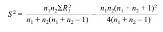To use the normal approximation when there are many ties, take

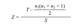
where S is the standard deviation for T and n₁(n₁ + n₂ + 1)/2 is the expected value of the rank sum under the null hypothesis. S is the square root of S², where

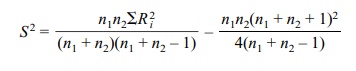
Here ΣR²_i is the sum of the squares of the ranks for all the data. This result is given in Conover (1999), page 273, using slightly different notation.

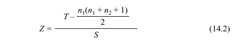
When there are no ties, Conover (1999) recommends a simpler approximation, namely,

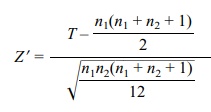
To summarize, Equation 14.1 describes the normal approximation for the Wilcoxon rank-sum test for comparing two independent samples (no ties) that can be used when n₁ and n₂ are large enough. Let T be the sum of the ranks for the pooled observations from one of the groups (samples). Then

where T is the sum of the ranks in one of the groups (e.g., control group) and n₁ and n₂ are, respectively, the sample sizes for samples from population 1 and population 2.

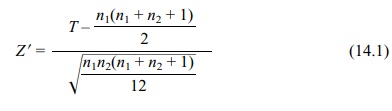
In the event of ties, the following normal approximation Wilcoxon rank-sum test for comparing two independent samples (ties) should be used when n₁ and n₂ are large enough (i.e., greater than 20). Let T be the sum of the ranks for the pooled ob-servations from one of the groups (samples). Then

where T is the sum of the ranks from one of the groups (e.g., control group); n₁ and n₂ are, respectively, the sample sizes for sample 1 and sample 2; and

where Σ^N_i=1R²_i is the sum of the squares of the ranks for all the data (N = n₁ + n₂). In the next two sections, we will look at the nonparametric analogs to the paired t test. They are the Wilcoxon signed-rank test (in Section 14.4) and the simpler but less powerful sign test (in Section 14.5).