Various approaches used for quantitative study of kinetic processes
| Home | | Biopharmaceutics and Pharmacokinetics |Chapter: Biopharmaceutics and Pharmacokinetics : Pharmacokinetics Basic Considerations
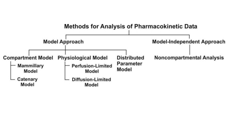
The two major approaches in the quantitative study of various kinetic processes of drug disposition in the body.
PHARMACOKINETIC ANALYSIS OF MATHEMATICAL DATA : PHARMACOKINETIC MODELS
Drug movement within the body is a complex process.
The major objective is therefore to develop a generalized and simple approach
to describe, analyse and interpret the data obtained during in vivo drug disposition studies. The
two major approaches in the quantitative study of various kinetic processes of
drug disposition in the body are (see Fig. 8.5) –
·
Model approach, and
·
Model-independent approach (also
called as non-compartmental analysis).
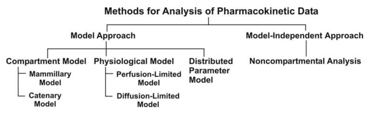
Fig. 8.5. Various approaches used for
quantitative study of kinetic processes
A. Pharmacokinetic Model Approach
In this approach, models are used to describe
changes in drug concentration in the body with time. A model is a hypothesis
that employs mathematical terms to concisely describe quantitative relationships. Pharmacokinetic models provide concise means of expressing mathematically or
quantitatively, the time course of drug(s) throughout the body and compute
meaningful pharmacokinetic parameters.
Applications of Pharmacokinetic
Models –
Pharmacokinetic models are useful in —
1.
Characterizing the behaviour of
drugs in patients.
2.
Predicting the concentration of
drug in various body fluids with any dosage regimen.
3.
Predicting the multiple-dose
concentration curves from single dose experiments.
4.
Calculating the optimum dosage
regimen for individual patients.
5.
Evaluating the risk of toxicity
with certain dosage regimens.
6.
Correlating plasma drug
concentration with pharmacological response.
7.
Evaluating the
bioequivalence/bioinequivalence between different formulations of the same
drug.
8.
Estimating the possibility of
drug and/or metabolite(s) accumulation in the body.
9.
Determining the influence of
altered physiology/disease state on drug ADME.
10. Explaining drug interactions.
Caution must however be exercised in ensuring that
the model fits the experimental data; otherwise, a new, more complex and
suitable model may be proposed and tested.
Types of Pharmacokinetic Models
Pharmacokinetic models are of three different types
–
1. Compartment models – are also called as empirical models, and
2. Physiological models – are realistic models.
3. Distributed parameter models – are also realistic
models.
1. Compartment Models
Compartmental analysis is the traditional and most
commonly used approach to pharmacokinetic characterization of a drug. These
models simply interpolate the experimental data and allow an empirical formula to estimate the drug
concentration with time.
Since compartments are hypothetical in nature,
compartment models are based on certain assumptions –
1. The body is represented as a
series of compartments arranged either in series or parallel to each other,
that communicate reversibly with each other.
2. Each compartment is not a real physiologic or
anatomic region but a fictitious or virtual one and considered as a tissue or
group of tissues that have similar drug distribution characteristics (similar blood
flow and affinity). This assumption is necessary because if every organ, tissue
or body fluid that can get equilibrated with the drug is considered as a
separate compartment, the body will comprise of infinite number of compartments
and mathematical description of such a model will be too complex.
3. Within each compartment, the
drug is considered to be rapidly and uniformly distributed i.e. the compartment
is well-stirred.
4. The rate of drug movement
between compartments (i.e. entry and exit) is described by first-order
kinetics.
5. Rate constants are used to
represent rate of entry into and exit from the compartment.
Depending upon whether the compartments are
arranged parallel or in a series, compartment models are divided into two
categories —
·
Mammillary model
·
Catenary model.
Mammillary Model
This model is the most common compartment model
used in pharmacokinetics. It consists of one or more peripheral compartments
connected to the central compartment in a manner similar to connection of
satellites to a planet (i.e. they are joined parallel to the central
compartment). The central compartment
(or compartment 1) comprises of plasma and highly perfused tissues such as lungs, liver, kidneys,
etc. which rapidly equilibrate with
the drug. The drug is directly absorbed into this compartment (i.e. blood).
Elimination too occurs from this compartment since the chief organs involved in
drug elimination are liver and kidneys, the highly perfused tissues and
therefore presumed to be rapidly accessible to drug in the systemic
circulation. The peripheral compartments or tissue compartments (denoted by numbers 2, 3, etc.) are
those with low vascularity and poor perfusion. Distribution of drugs to these
compartments is through blood.
Movement of drug between compartments is defined by characteristic first-order
rate constants denoted by letter K (see
Fig. 8.6). The subscript indicates the direction of drug movement; thus, K12
(K-one-two) refers to drug movement from compartment 1 to compartment 2 and
reverse for K21.
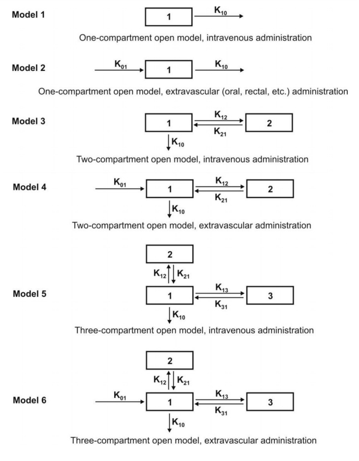
Fig. 8.6. Various mammillary compartment models. The rate constant K01 is
basically Ka, the first-order
absorption rate constant and K10 is KE, the first-order elimination rate
constant.
The number of rate constants which will appear in a
particular compartment model is given by R.
For intravenous administration, R = 2n – 1 (8.17)
For extravascular administration, R = 2n (8.18)
where n = number of compartments.
Catenary Model
In this model, the compartments are joined to one
another in a series like compartments of a train (Fig. 8.7). This is however
not observable physiologically/anatomically as the various organs are directly
linked to the blood compartment. Hence this model is rarely used.
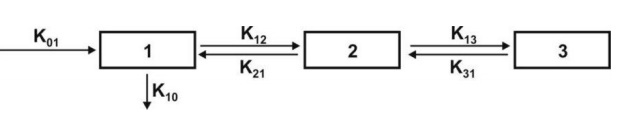
Fig. 8.7. A catenary model
The compartment modelling approach has several advantages and applications —
1. It is a simple and flexible
approach and thus widely used. Fundamentally, the principal use of this
approach is to account for the mass balance of drug in plasma, drug in
extravascular tissues and the amount of drug eliminated after its
administration. It often serves as a ―first-model‖.
2. It gives a visual
representation of various rate processes involved in drug disposition.
3. It shows how many rate
constants are necessary to describe these processes.
4. It enables the
pharmacokineticist to write differential equations for each of the rate
processes in order to describe drug-concentration changes in each compartment.
5. It enables monitoring of drug
concentration change with time with a limited amount of data. Only plasma
concentration data or urinary excretion data is sufficient.
6. It is useful in predicting
drug concentration-time profile in both normal physiological and in
pathological conditions.
7. It is important in the development of dosage
regimens.
8. It is useful in relating
plasma drug levels to therapeutic and toxic effects in the body.
9. It is particularly useful when
several therapeutic agents are compared. Clinically, drug data comparisons are
based on compartment models.
10. Its simplicity allows for
easy tabulation of parameters such as Vd, t½, etc.
Disadvantages of compartment modelling include —
1. The compartments and
parameters bear no relationship with the physiological functions or the anatomic
structure of the species; several assumptions have to be made to facilitate
data interpretation.
2. Extensive efforts are required
in the development of an exact model that predicts and describes correctly the
ADME of a certain drug.
3. The model is based on curve
fitting of plasma concentration with complex multiexponential mathematical
equations.
4. The model may vary within a
study population.
5. The approach can be applied
only to a specific drug under study.
6. The drug behaviour within the
body may fit different compartmental models depending upon the route of
administration.
7. Difficulties generally arise
when using models to interpret the differences between results from human and
animal experiments.
8. Owing to their simplicity,
compartmental models are often misunderstood, overstretched or even abused.
Because of the several drawbacks of and
difficulties with the classical compartment modelling, newer approaches have
been devised to study the time course of drugs in the body. They are — physiological
models and noncompartmental methods.
2. Physiological Models
These models are also known as physiologically-based pharmacokinetic models (PB-PK models).
They are drawn on the basis of known anatomic and physiological data and thus present
a more realistic picture of drug disposition in various organs and tissues. The
number of compartments to be included in the model depends upon the disposition
characteristics of the drug. Organs or tissues such as bones that have no drug
penetration are excluded. Since describing each organ/tissue with mathematic
equations makes the model complex, tissues with similar perfusion properties
are grouped into a single compartment. For example, lungs, liver, brain and
kidney are grouped as rapidly equilibrating tissues (RET) while muscles and
adipose as slowly equilibrating tissues (SET). Fig. 8.8 shows such a
physiological model where the compartments are arranged in a series in a flow
diagram.
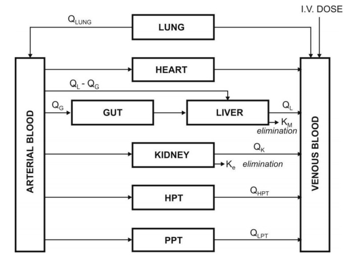
Fig. 8.8. Schematic representation of a
physiological pharmacokinetic model. The term Q indicates blood flow rate to a body region. HPT stands for other
highly perfused tissues and PPT for poorly perfused tissues. Km is rate
constant for hepatic elimination and Ke is first-order rate constant for
urinary excretion.
Since the rate of drug carried to a tissue organ
and tissue drug uptake are dependent upon two major factors –
·
Rate of blood flow to the organ,
and
·
Tissue/blood partition
coefficient or diffusion coefficient of drug that governs its tissue permeability,
The physiological models are further categorized
into two types –
1. Blood flow rate-limited models – These models are more popular and
commonly used than the second type,
and are based on the assumption that the drug movement within a body region is
much more rapid than its rate of delivery to that region by the perfusing
blood. These models are therefore also called as perfusion rate-limited models.
This assumption is however applicable only to the highly membrane
permeable drugs i.e. low molecular weight, poorly ionised and highly lipophilic
drugs, for example, thiopental, lidocaine, etc.
2. Membrane permeation rate-limited models – These models are more
complex and applicable to highly
polar, ionised and charged drugs, in which case the cell membrane acts as a
barrier for the drug that gradually permeates by diffusion. These models are
therefore also called as diffusion-limited models. Owing to
the time lag in equilibration between the blood and the tissue, equations for
these models are very complicated.
Physiological modelling has several advantages over the conventional
compartment modelling –
1.
Mathematical treatment is
straightforward.
2.
Since it is a realistic approach,
the model is suitable where tissue drug concentration and binding are known.
3.
Data fitting is not required
since drug concentration in various body regions can be predicted on the basis
of organ or tissue size, perfusion rate and experimentally determined
tissue-to-plasma partition coefficient.
4.
The model gives exact description
of drug concentration-time profile in any organ or tissue and thus better
picture of drug distribution characteristics in the body.
5.
The influence of altered
physiology or pathology on drug disposition can be easily predicted from
changes in the various pharmacokinetic parameters since the parameters
correspond to actual physiological and anatomic measures.
6.
The method is frequently used in
animals because invasive methods can be used to collect tissue samples.
7.
Correlation of data in several
animal species is possible and with some drugs, can be extrapolated to humans
since tissue concentration of drugs is known.
8.
Mechanism of ADME of drug can be
easily explained by this model.
Disadvantages of physiological modelling
include —
1.
Obtaining the experimental data
is a very exhaustive process.
2.
Most physiological models assume
an average blood flow for individual subjects and hence prediction of
individualized dosing is difficult.
3.
The number of data points is less
than the pharmacokinetic parameters to be assessed.
4.
Monitoring of drug concentration
in body is difficult since exhaustive data is required
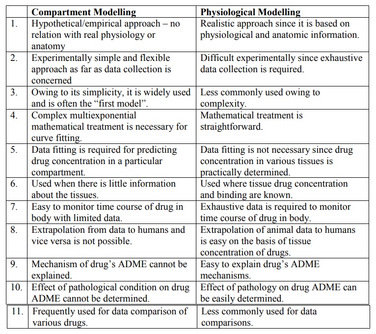
Table 8.1 briefly compares features of compartment
and physiological models.
TABLE 8.1. Comparison of features of compartment and physiological
models
Compartment Modelling
1.
Hypothetical/empirical approach –
no relation with real physiology or anatomy
2.
Experimentally simple and
flexible approach as far as data collection is concerned
3.
Owing to its simplicity, it is
widely used and is often the ―first model‖.
4.
Complex multiexponential
mathematical treatment is necessary for curve fitting.
5.
Data fitting is required for
predicting drug concentration in a particular compartment.
6.
Used when there is little
information about the tissues.
7.
Easy to monitor time course of
drug in body with limited data.
8.
Extrapolation from data to humans
and vice versa is not possible.
9.
Mechanism of drug’s ADME cannot
be explained.
10. Effect of pathological condition on drug ADME cannot be determined.
11. Frequently used for data comparison of various drugs.
Physiological Modelling
1.
Realistic approach since it is
based on physiological and anatomic information.
2.
Difficult experimentally since
exhaustive data collection is required.
3.
Less commonly used owing to
complexity.
4.
Mathematical treatment is
straightforward.
5.
Data fitting is not necessary
since drug concentration in various tissues is practically determined.
6.
Used where tissue drug
concentration and binding are known.
7.
Exhaustive data is required to
monitor time course of drug in body.
8.
Extrapolation of animal data to
humans is easy on the basis of tissue concentration of drugs.
9.
Easy to explain drug’s ADME
mechanisms.
10. Effect of pathology on drug ADME can be easily determined.
11. Less commonly used for data comparisons.
3. Distributed Parameter Model
This model is analogous to physiological model but
has been designed to take into account –
·
Variations in blood flow to an
organ, and
·
Variations in drug diffusion in
an organ.
Such a model is thus specifically useful for
assessing regional differences in drug concentrations in tumours or necrotic
tissues.
The distributed parameter model differs from
physiological models in that the mathematical equations are more complex and
collection of drug concentration data is more difficult.
B. Noncompartmental Analysis
The noncompartmental analysis, also
called as the model-independent method,
does not require the assumption of specific compartment model. This method is,
however, based on the assumption that the
drugs or metabolites follow linear kinetics, and on this basis, this technique can be applied to
any compartment model.
The noncompartmental approach, based on the statistical moments theory, involves collection of
experimental data following a single dose of drug. If one considers the time
course of drug concentration in plasma as a statistical distribution curve,
then:
MRT = AUMC/AUC (9.19)
where
MRT = mean residence time
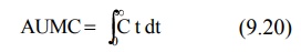
AUMC = area under the first-moment curve
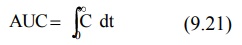
AUC = area under the zero-moment curve
AUMC is obtained from a plot of product of plasma
drug concentration and time (i.e. C.t) versus time t from zero to infinity
(Fig. 8.9). Mathematically, it is expressed by equation:
AUC is obtained from a plot of plasma drug
concentration versus time from zero to infinity. Mathematically, it is
expressed by equation:
Practically, the AUMC and AUC can be calculated
from the respective graphs by the trapezoidal
rule (the method involves dividing the curve by a series of vertical lines
into a number of trapezoids,
calculating separately the area of each trapezoid and adding them together).
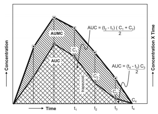
Fig. 8.9. AUC and AUMC plots
MRT is defined as the average amount of time spent by the drug in the body
before being eliminated. In this sense, it is the statistical moment analogy of half-life, t½.
In effect, MRT represents the time
for 63.2% of the intravenous bolus dose to be eliminated. The values will
always be greater when the drug is administered in a fashion other than i.v.
bolus.
Applications of noncompartmental technique
includes –
1. It is widely used to estimate the important
pharmacokinetic parameters like bioavailability, clearance and apparent volume
of distribution.
2. The method is also useful in
determining half-life, rate of absorption and first-order absorption rate
constant of the drug.
Advantages of noncompartmental method
include —
1. Ease of derivation of
pharmacokinetic parameters by simple algebraic equations.
2. The same mathematical
treatment can be applied to almost any drug or metabolite provided they follow
first-order kinetics.
3. A detailed description of drug
disposition characteristics is not required.
Disadvantages of this method include –
1. It provides limited
information regarding the plasma drug concentration-time profile. More often,
it deals with averages.
2. The method does not adequately treat non-linear
cases.
Related Topics

