The Binomial Distribution

THE BINOMIAL DISTRIBUTION

As introduced in the previous section, the binomial random variable is the count of the number of successes in n independent trials when the probability of success on any given trial is p. The binomial distribution applies in situations where there are only two possible outcomes, denoted as S for success and F for failure.

Each such trial is called a Bernoulli trial. For convenience, we let X_i be a Bernoulli random variable for trial i. Such a random variable is assigned the value 1 if the trial is a success and the value 0 if the trial is a failure.

For Z (the number of successes in n trials) to be Bi(n, p), we must have n inde-pendent Bernoulli trials with each trial having the same probability of success p. Z then can be represented as the sum of the n independent Bernoulli random variables X_i for i = 1, 2, 3, . . . , n. This representation is convenient and conceptually impor-tant when we are considering the Central Limit Theorem (discussed in Chapter 7) and the normal distribution approximation to the binomial.

The binomial distribution arises naturally in many problems. It may represent appropriately the distribution of the number of boys in families of size 3, 4, or 5, for example, or the number of heads when a coin is flipped n times. It could represent the number of successful ablation procedures in a clinical trial. It might represent the number of wins that your favorite baseball team achieves this season or the number of hits your favorite batter gets in his first 100 at bats.

Now we will derive the general binomial distribution, Bi(n, p). We simply gener-alize the combinatorial arguments we used in the previous section for Bi(3, 0.50). We consider P(Z = r) where 0 ≤ r ≤ n. The number of elementary events that lead to r successes out of n trials (i.e., getting exactly r successes and n – r failures) is C(n, r) = n!/[(n – r)! r!].

Recall our earlier example of filling slots. Applying that example to the present situation, we note that one such outcome that leads to r successes and n – r failures would be to have the r successes in the first r slots and the n – r failures in the re-maining n – r slots. For each slot, the probability of a success is p, and the probabil-ity of a failure is 1 – p. Given that the events are independent from trial to trial, the multiplication rule for independent events applies, i.e., products of terms which are either p or 1 – p. We see that for this particular arrangement, p is multiplied r times and 1 – p is multiplied n – r times.

The probability for a success on each of the first r trials and a failure on each of the remaining trials is p^r(1 – p)^n–r. The same argument could be made for any other arrangement. The quantity p will appear r times in the product and 1 – p will appear n – r times. The product of multiplication does not change when the order of the terms is changed. Therefore, each arrangement of the r successes and n – r failures has the same probability of occurrence as the one that we just computed.

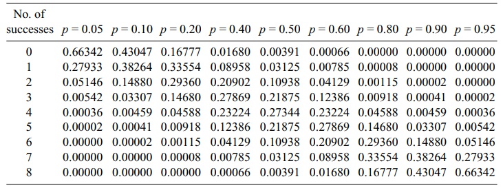
TABLE 5.2. Binomial Distributions for n = 8 and p ranging from 0.05 to 0.95

The number of such arrangements is just the number of ways to select exactly r out of the n slots for success. This number denotes combinations for selecting r objects out of n, namely, C(n, r). Therefore, P(Z = r) = C(n, r)(1 – p)^n–r = {n!/[r!(n – r)!]}p^r(1 – p)^n–r. Because the formula for P(Z = r) applies for any value of r between 0 and n (including both 0 and n), we have the general binomial distribution.

Table 5.2 shows for n = 8 how the binomial distribution changes as p ranges from small values such as 0.05 to large values such as 0.95. From the table, we can see the relationship between the probability distribution for Bi(n, p) and the one for Bi(n, 1 – p). We will derive this relationship algebraically using the formula for P(Z = r).

Suppose Z has the distribution Bi(n, p); then P(Z = r) = n!/[(n – r)!r!]p^r(1 – p)^n–r. Now suppose W has the distribution Bi(n, 1 – p). Let us consider P(W = n – r). P(W = n – r) = n!/[{n – (n – r)}!(n – r)!](1 – p)^n–rp^r = n!/[r! (n – r)!](1 – p)^n–rp^r. Without changing the product, we can switch terms around in the numerator and switch terms around in the denominator: P(W = n – r) = n!/[r! (n – r)!](1 – p)^n–r p^r = n!/[(n – r)! r!]p^r(1 – p)^n–r. But we recognize that the term on the far-right-hand side of the chain of equalities equals P(Z = r). So P(W = n – r) = P(Z = r). Consequently, for 0 ≤ r ≤ n, the probability that a Bi(n, p) random variable equals r is the same as the probability that a Bi(n, 1 – p) random variable is equal to n – r.

Earlier in this chapter, we noted that Bi(n, p) has a mean of μ = np and a variance of σ² = npq, where q = 1 – p. Now that you know the probability mass function for the Bi(n, p), you should be able to verify these results in Exercise 5.21.