Tests of statistical significance

Tests of statistical significance

The need for the statistical tests of significance is exemplified by questions posed in comparing two data sets. The tests of statistical significance are intended to compare two sets of data to address the question whether these data sets represent two different populations, that is, whether they are inherently different or not. A data set is a sample presumed to be taken from an infinite population of data that would represent infinite repeti-tions of the experiment. If two samples are taken from the same popula-tion, they would have a greater overlap with each other than if the samples belong to two different populations. As shown in Figure 5.7, samples 1 and 2 apparently come from two different populations in subfigure A but not in subfigure B. However, it is difficult to comment on whether the samples come from different populations in subfigure C. The tests of statistical sig-nificance are designed to answer questions such as these.

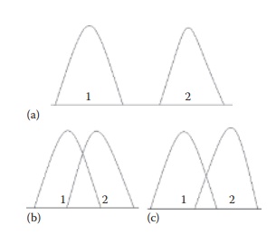
Figure 5.7 Three scenarios that may be encountered when comparing data sets from two samples, 1 and 2. In case A, the sample values of the two samples are significantly different by a large numeric value, indicating that the samples most likely represent two different populations. In case B, the sample values are so close to each other that it is very likely that both samples came from the same population and are not different from each other. In case C, the differences in sample values are intermediate. In the case of scenario C, it is difficult to make an assessment whether the two samples are really different from each other. In such cases, the tests of significance provide a statistical basis for decision making.

Parametric and nonparametric tests

A sample or a population can be described by the mean and variance of all observations, which represent statistical parameters, with an assumption of a known underlying population distribution. Alternatively, a nonparametric measure, such as median, can be used, which assume an underlying popula-tion distribution but not necessarily a known distribution.

Accordingly, statistical tests of significance can be parametric or nonparametric:

·           Parametric tests of significance are based on parametric measures of distribution of data, viz., mean and variance of the data set. They assume a specific and known distribution of the underlying population.

·           Nonparametric tests of significance are based on nonparametric descriptors of distribution of data, viz., median and ranks of the data values. They do not make the assumption about that the underlying distribution of the population is known.

Parametric tests are more powerful (less probability of type II error, described later) than the nonparametric tests, since they use more information about the samples. They are frequently used to provide information, such as inter-action between two variables in a factorial design of experiments. However, they are also more sensitive to skewness in the distribution of data and the presence of outliers in the samples. Therefore, nonparametric tests may be preferred for skewed distributions.

Parametric tests are exemplified by t-test, chi square test, and analysis of variance (ANOVA). Nonparametric tests are exemplified by Wilcoxon, Kruskal– Wallis, and Mann– Whitney tests. The parametric tests will be described in more detail in the following sections.

Null and alternate hypothesis

Statistical tests of significance are designed to answer this and similar ques-tions with a given level of confidence and power, expressed in numerical terms. Statistical tests of significance can be used, for example, to test the hypothesis that (a) a sampled data set comes from a single population or that (b) two sampled data sets come from a single population. A statistical hypothesis represents an assumption about a population parameter. This assumption may or may not be true and is sought to be tested using the sta-tistical parameters obtained from a sample. For example, if the statistical tests of significance test the hypothesis that a given variation within or among data sets occurred purely by chance, it would be termed the null hypothesis. In this case, therefore, the null hypothesis is the hypothesis of no difference. If the null hypothesis cannot be proven at the selected levels of confidence and power of the test, the alternate hypothesis is assumed to hold true. The alternate hypothesis indicates that the sample observations are influenced by some nonrandom cause.

Steps of hypothesis testing

The process of testing a hypothesis involves the following general steps:

1.        Ask the question (for a practical situation) that can be addressed using one of the statistical tests of significance.

2.        Select the appropriate test of significance to be used and verify the validity of underlying assumptions.

3.        State null and alternate hypothesis.

4.        Define significance level (e.g., α = 0.01, 0.05, or 0.1, which indicates 1%, 5%, or 10% probability of occurrence of given differences just by chance). Lower the significance level, greater the chance of not detecting the differences when they actually do exist.

5.        Define sample size. Sample size affects the power of the significance test. Higher the sample size, higher the power, that is, greater the chance of detecting the differences when they actually do exist.

6.        Compute the test statistic.

7.        Identify the probability (p) of obtaining a test statistic as extreme as the calculated test statistic for the calculated degrees of freedom, using standard probability distribution tables.

8.        Compare this probability with the level of significance desired. If p_{sample at α} < p, null hypothesis is rejected. If p_{sample at α} ≥ p, null hypothesis cannot be rejected.

One-tailed and two-tailed hypothesis tests

The null and alternate hypotheses can be stated such that the null hypoth-esis is rejected when the test statistic is higher or lower than a given value, or both. The first two are called one-tailed hypothesis, while the latter is termed two-tailed hypothesis. For example, if μ₁ and μ₂ represent the means of two populations and H₀ represents the null hypothesis, (H₀: μ₁ − μ₂ ≥ d) or (H₀: μ₁ − μ₂ ≤ d) would be one-tailed hypothesis, since H₀ would be rejected when (μ₁ − μ₂ < d) and (μ₁ − μ₂ > d), respectively. However, (H₀: μ₁ − μ₂ = d) is a two-tailed hypothesis, since the null hypothesis would be rejected in both cases of (μ₁ − μ₂ < d) and (μ₁ − μ₂ > d).

The appropriate statement of null hypothesis depends on the practical situation being addressed. For example,

·           If a sample of tablets were collected during a production run of tablet-ing unit operation and tested for average tablet weight, the question could be asked whether the average tablet weight is the target tab-let weight. In this case: (H₀: Weight_sample − Weight_target = 0) or (H₀: Weight_sample = Weight_target) would be a two-tailed hypothesis test, since the null hypothesis would be rejected when the sample weight is both higher than or lower than the target weight.

·           If a sample of tablets were collected during a production run of the coating unit operation and tested for coating weight build-up on the tablets, the question could be asked whether the coating weight build-up has reached the target weight build-up of 3% w/w. In this case: (H₀: Weight_sample – Weight_target ≥ 0) would be a one-tailed hypothesis test, since the null hypothesis would be rejected only if the sample weight is less than the target weight.

Regions of acceptance and rejection

The regions of acceptance and rejection of a hypothesis refer to regions in the probability distribution of the sample’s test statistic. Assuming that the null hypothesis is true, a sample’s test statistic is normally distributed, with the shape of the distribution defined by the degrees of freedom of the sample. Therefore, the probability of finding a given value of the test statistic can be defined by this distribution curve. For example, Figure 5.8a shows the nor-mal distribution of a test statistic, with a vertical line to the right indicating the value of the test statistic associated with a probability of occurrence (α) of 0.05, or 5%, by random chance, or P_α. Decreasing the level of signifi-cance (α) increases the rigor of the test; that is, the differences must be really significant to be detected.

For a one-tailed hypothesis test (Figure 5.8a), the region of rejection lies on one (right) side of this distribution. If the test statistic value obtained for the sample in question is higher than P_α , the test statistic in the sample is assumed to lie in the region of rejection and the null hypothesis is rejected at the chosen level of significance (α). Region of acceptance in this case is defined as (−∞ to P_α).

For a two-tailed hypothesis test (Figure 5.8b), the region of rejection lies on either side of the distribution. If the test statistic value obtained for the sample in question is higher than P_α or lower than −P_α , the test statistic in the sample is assumed to lie in the region of rejection and the null hypoth-esis is rejected at the chosen level of significance (α). Region of acceptance in this case is defined as (−P_α to P_α).

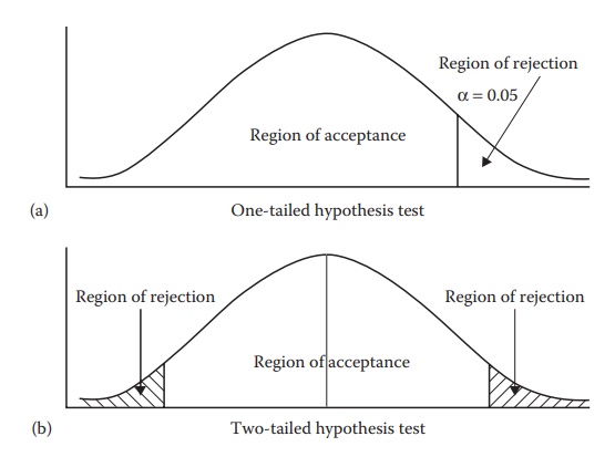
Figure 5.8 An illustration of regions of acceptance and rejection in a normal probability distribution. Knowing the probability of occurrence of sample values at either extremes from the mean as a function of the standard deviation (Figure 5.6), a given level of significance (e.g., α = 0.05) can quantify a cut-off point, indicated by a vertical line in the plot. This vertical line in Figure 5.8a represents 5% chance of occurrence of data values. Therefore, any value higher than the indicated α line has a lower than 5% chance of occurrence and is said to fail in the region of rejection. This is one-tailed hypothesis, since data values on only one side of the mean are being considered for hypothesis testing. This side could be the positive side, as indicated in Figure 5.8a, or the negative side, which would be indicated by the α line on the left of the mean. In a two-tailed hypothesis testing (Figure 5.8b), data values on both positive and negative sides of the mean are considered. Data values that are more extreme than the α line are said to fall in the region of rejection. All other data values are considered in the region of acceptance.

Probability value and power of a test

The level of significance of test results is indicated by the probability value (abbreviated as p-value). The p-value is the fractional probability of accepting the null hypothesis, assuming that the null hypothesis is true. In other words, lower the p-value of the test, expressed as fractional prob-ability (e.g., 0.01, 0.05, or 0.1, representing 1%, 5%, or 10% probability, respectively), greater the chance of accepting the null hypothesis and not detecting differences between two samples. Lower p-value indicates greater difference between two samples. The commonly used probability level for accepting the null hypothesis is 5%, corresponding to the p-value of 0.05.

The power of a test of significance is the probability of rejecting the null hypothesis, assuming that the null hypothesis is not true. In other words, higher the power of the test, expressed in %, greater the chance that true differences between two different sample sets would be detected. Power of a test can be increased by increasing the sample size. The commonly accepted power of a test is 80%.

Types of error

Conducting a test of significance can result in two types of errors in assessing the difference in the chosen test statistic:

·           Type I error is a false positive in finding the difference and inappro-priately rejected null hypothesis. This is the error of rejecting a null hypothesis when it is actually true. In other words, type I error is the error of finding the difference between the two samples when they are actually not different. The probability of type I error is denoted by α.

The probability of type I error is higher when the chosen level of significance, α, is higher. Therefore, using lower α tends to reduce the probability of a type I error.

·           Type II error is a false negative in finding the difference and inappro-priately failing to reject null hypothesis. This is the error of not reject-ing a null hypothesis when it is actually not true. In other words, type II error is the error of not finding difference between the two samples when they are actually different. The probability of type II error is denoted by β.

The probability of type II error is higher when the chosen power of the test, β, is lower. Therefore, using higher β tends to reduce the probability of a type II error.

Questions addressed by tests of significance

Tests of significance are designed to answer specific types of questions based on a selected test statistic and a probability distribution of the test statistic. For example, the differences between means are tested using t-test, the dif-ferences between proportions are tested using z-test, and the differences in the frequency of a categorical variable are tested using χ² test. Commonly used tests of significance, an example situation, underlying assumptions of tests, statement of null hypothesis, and calculations of the test statistic are summarized in Table 5.6.

Table 5.6 Statistical tests of significance

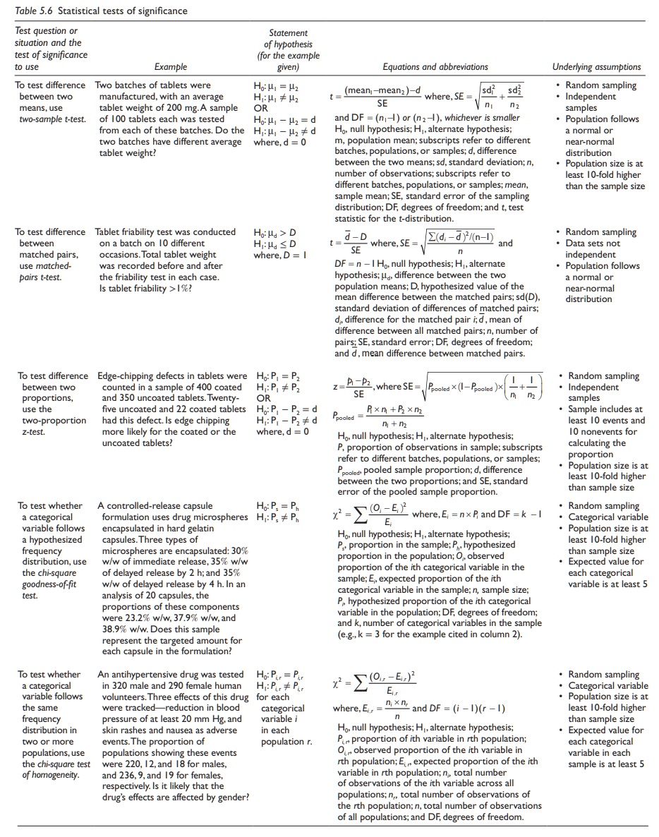
It should be noted that these tests of significance invariably involve:

·           The calculation of a test statistic, which represents the difference between the expected and the observed values, or the values of two samples. It also takes into account the variability in the sample through incorporation of standard error. The calculation of test statistic involves quantifying the extent of observed differences vis-à-vis the variability.

·           Identifying the probability value associated with the test statistic at a given level of significance (P_α) for the given degrees of freedom. The degree of freedom is calculated based on the sample size and sometimes also the number of variables studied. The degrees of freedom affect the distribution plot of the test statistic and thus the P_α value for a given α.

Having calculated the P_α value and the test statistic, the given test of signifi-cance is carried out per the steps outlined earlier. For example, if the value of test statistic obtained for a given test of significance is 0.942 and the P_α value at the desired probability of error of 5% is 1.347, the test statistic falls in the region of acceptance. Hence, the null hypothesis cannot be rejected. On the other hand, if the test statistic value were higher than 1.347, the test statistic would fall in the region of rejection. Hence, the null hypothesis would be rejected.

Analysis of variance

The analysis of variance uses differences between means and variances to quantify statistical significance between means of different samples. Any number of samples or subgroups may be compared in an ANOVA experiment. ANOVA is based on the underlying explanation of variation of sample values from the population mean as being a linear combination of the variable effect and random error.

The number of variables (also termed treatments or factors) in an ANOVA experiment can be one (one-way ANOVA), two (two-way ANOVA), or more. Each variable or factor can be studied at different levels, indicating the intensity. For example, a clinical study that evaluates one dose of an experimental drug is a one-variable one-level experiment. A study that eval-uates two doses of an experimental drug would be a one-variable two-level study. Another study that evaluates three doses of two experimental drugs would be a two-variable three-level study. The level may be a quantitative number, such as the dose in the above examples, or it may be a numerical designation of the presence or intensity of an effect, such as “0” and “1.”

1. One-way ANOVA

 Model equation

When sample sets are treated with a single variable at i different levels (i = 1, 2, 3, …, k), the value of each data point is explained as:

y_ij = µ + τ_i + ε_ij

where:

y_ij represents the jth observation of the ith level of treatment of the variable

μ is the mean of all samples in the experiment

τ_i is the ith treatment effect

ε_ij represents random error

Hence, the value of each data point in an experiment is represented in terms of the mean of all samples and deviations arising from the effect of treat-ment or variable being studied (τ_i) and random variation (ε_ij). This equation represents a one-way ANOVA model.

Underlying assumptions

ANOVA is used to test hypotheses regarding means of two or more samples, assuming the following:

·           The underlying populations are normally distributed.

·           Variances of the underlying populations are approximately equal.

·           The errors (ε_ij) are random and have a normal and independent distri-bution, with a mean of zero and a variance of σ²_ε .

Fixed- and random-effects model

The one-way ANOVA model quantifies variation in each data point (y_ij) from the mean of all data points (μ) as a combination of random variation (ε_ij) and the effect of a known variable or treatment (τ). Different subgroups of the experimental data points can be subjected to different levels of the treatment, τ_i, where i = 1, 2, 3, … k. If the levels of the treatment are fixed, the model is termed fixed-effects model. On the other hand, if the levels of the treatment are randomly assigned from several possible levels, the model is termed random-effects model.

Whether the levels of a variable or treatment are fixed or random depends on the design of the experiment. A fixed effects model is exemplified by three subgroups of a group of 18 volunteers chosen for a pharmacokinetic study of a given drug at dose levels of 0, 50, and 100 mg. A random effects model would be exemplified by three subgroups of a group of 18 volunteers chosen for a pharmacokinetic study of three different drugs A, B, and C at unknown and variable dose levels (e.g., dose titration by the physician for individualization to the patient). The effects are assumed to be random in the latter case, since the level of the drug is not fixed.

The selection of a study design as a fixed- or random-effects model is criti-cal to the accuracy of data interpretation. The calculation of variance between treatment groups is different between fixed- and random-effects model.

Null and alternate hypothesis

The null hypothesis (H₀) for a one-way ANOVA experiment would be no difference between the population means of samples treated with different levels of the selected factor. The alternate hypothesis (H₁) states that the means of underlying populations are not equal.

Calculations for fixed-effects model from first principles

ANOVA is based on the calculation of ratio of variance introduced by the factor and random variations. Although many software tools are currently available that reduce the requirement for tedious calculations, it is impor-tant to understand the calculations of statistical tests of significance from first principles.

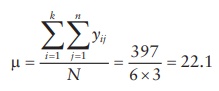
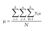
1. Mean of all samples in the experiment (μ) is calculated by adding all observations and dividing by the total number of samples in the experiment.

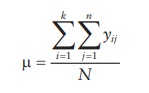
where, y_ij represents the jth observation of the ith level of treatment of the variable, there being a total of k treatments (i = 1, 2, 3, … k) and n samples per treatment level (j = 1, 2, 3, …. n), and N being the total n sample size, including all treatments and levels.

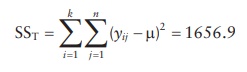
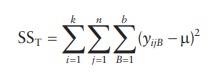
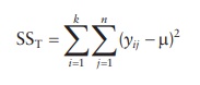
2. Total sum of squares (SS_T) of all observations is calculated by squaring all observations and subtracting from the mean of all samples in the experiment (μ).

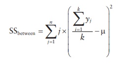
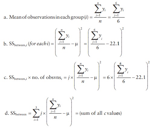
3. Sum of squares for the factor studied is the sum of squares between the columns (SS_between) if each level of the factor is arranged in a col-umn. It is calculated by subtracting the mean value for each column from the mean of all samples, squaring this value, and adding for all columns.

4. Sum of squares for the random error (SS_error) is the difference between the total sum of squares and the sum of squares between and within the columns.

SS_error = SS_total − SS_between

5. Degrees of freedom are calculated as follows:

Degrees of freedom between groups (DF_between):

DF_between = k − 1

Degrees of freedom for the error term (DF_error):

DF_error = N − k

6. Mean squares for the random error (MS_error) and the factor studied (MS_between) are calculated by dividing their respective sum of squares by their DF.

MS_between = SS_between /DF_between

MS_error = SS_error/DF_error

7. An F-ratio is computed as the ratio of mean squares of factor effect to the mean square of error effect.

F = MS_between / MS_error

8. Determine critical F-ratio at (DF_between and DF_error) degrees of freedom for α = 0.05.

9. Test the hypothesis. The F-ratio is compared to the P_α value for the F-test at designated degrees of freedom to determine the signifi-cance of observed results. Statistical significance of results would indicate that the contribution of the factor’s or variable’s effect on the observations is significantly greater than the variation that can be ascribed to random error.

Example of calculations for fixed-effects model

The computation of statistical significance by one-way ANOVA can be illus-trated by a case of administration of two doses of a test antihyperlipidemic compound and a placebo to a set of six patients in each group. Hypothetical results of this study in terms of reduction of blood cholesterol level are summarized in Table 5.7. These data can be rephrased in statistical terms, as presented in Table 5.8.

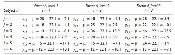
Table 5.7 A hypothetical example of a one-way ANOVA experiment

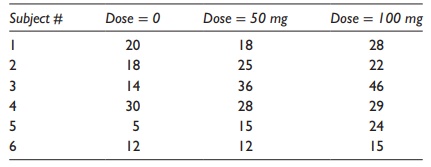
Table 5.8 Rephrasing the data in statistical terms for a hypothetical example of a one-way ANOVA experiment

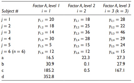
1. Mean of all samples in the experiment (μ):

2. Total sum of squares of variation in all data points (SS_T): The calculations are illustrated in Table 5.9.

Squaring (y_ij-μ) values and adding them together,

3. Sum of squares of variation coming from the factor studied (SS_between): As calculated in Table 5.8.

4. Sum of squares of variation coming from random error (SS_error): As calculated in Table 5.8.

SS_total = S_between + SS_error

SS_error = SS_total − SS_between

SS_error = 1656.9 − 352.8 = 1304.2

5. Degrees of freedom (DF):

Degrees of freedom between groups (DF_between):

DF_between = k − 1 = 3 − 1 = 2

Table 5.9 Calculations for a hypothetical example of a one-way ANOVA experiment

Degrees of freedom for the error term (DF_error):

DF_error = N − k = 18 − 3 = 15

6. Mean squares (MS) of variation:

Mean square between groups (MS_between):

MS_between = SS_between / DF_between = 352.8/2 = 176.4

Mean square for the error term (MS_error):

MS_error = SS_error/ DF_error = 1304.2/15 = 86.9

7. F-ratio:

F = MS_between / MS_error = 176.4/86.9 = 2 .0

8. Determine the critical F-ratio at the chosen P_α value. Determine the critical F-ratio at (2, 15) degrees of freedom for α = 0.05 is 3.7.

9. Test the hypothesis: Since the obtained F-value is lower than the criti-cal F-value, the null hypothesis (no difference) cannot be rejected. In this example, although the data do look significantly different when reviewed without statistical analysis, the high random error in the observations leads to lack of statistical significance.

An alternate means to test the hypothesis is to use the standard tables to determine the p-value associated with the observed F-value. If the observed p-value is less than the chosen P_α value (e.g., 0.05), the null hypothesis is rejected. For example, in the above calculations, the p-value associated with the observed F-ratio is 0.17. Since this is higher than 0.05, the null hypothesis cannot be rejected.

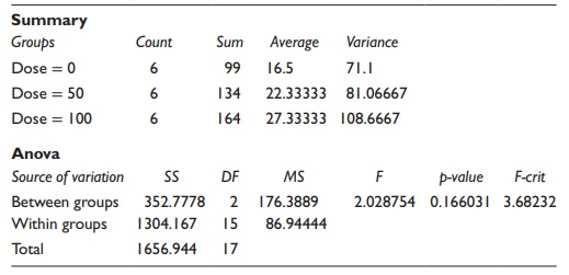
Calculations using Microsoft Excel

An alternate to calculations from first principles is to use one of the available software tools for calculations. As an illustration, when Microsoft Excel’s data analysis add-in function is utilized for single-factor ANOVA calcula-tions, the software provides a tabular output of calculated values illustrated in Table 5.10.

This tabular output of results summarizes statistical parameters associ-ated with the data, followed by a summary of calculated results in a tabular format. The critical F-value and the p-value associated with the calculated F-value are indicated to facilitate hypothesis testing.

Table 5.10 Statistical results for a hypothetical example of a one-way ANOVA experiment using Microsoft Excel

2. Two-way ANOVA: Design of experiments

Two-way ANOVA deals with investigation of effects of two variables in a set of experiments. ANOVA with two or more variables (also called treat-ments or factors) is most commonly utilized in the design of experiments.

Factorial experiments

When the effects of more than one factor are studied at one or more levels, the factorial experiment is defined as an L^F-factorial experiment. For exam-ple, three factors evaluated at two different levels would be a 2³ factorial experiment and two factors evaluated at three different levels would be a 3² experiment. An example of such studies is the effect of temperature and pres-sure on the progress of a reaction. If an experiment is run at two temperature and pressure values, it is a 2² factorial experiment, with the total number of runs = 2 × 2 = 4. If the experiment were run at three levels of temperature and pressure, it would be a 3² factorial experiment, with the total number of experimental runs = 3 × 3 = 9. Conversely, if three factors (e.g., tempera-ture, pressure, and reactant concentration) were studied at two levels each, it would be a 2³ factorial experiment, with 2 × 2 2 = 8 experimental runs. The experiments could be full-factorial or partial-factorial.

·           A full-factorial experiment is one in which all combinations of all fac-tors and levels are studied. For example, a full-factorial four-factor, two-level study would involve 2⁴ = 2 × 2 × 2 × 2 = 16 experimental runs. Full-factorial experiments provide information on both the main effects of various factors and the effects of their interactions. Design and interpretation of a two-factor, two-level experiment are illustrated in the two-way ANOVA model.

·           A partial-factorial experiment is one in which half the combinations of levels of all factors are studied. For example, a partial-factorial four-factor, two-level study would involve 2⁴⁻¹ = 16/2 = 8 experi-mental runs. Partial-factorial experiments provide information on the main effects of various factors but not on the interaction effects. Design and interpretation of partial-factorial experiments are beyond the scope of this chapter.

Model equation

If there are two variables or treatments being studied in the experiment, the value of each data point is explained as:

y_ijk = µ + τ_i + β _j + γ_ij + ε_ijk

where:

y_ijk represents the jth observation of the ith level of treatment of the first variable and kth treatment of the second variable

μ is the mean of all samples in the experiment

τ_i is the ith treatment effect of the first variable

β_j is the jth treatment effect of the second variable

ε_ijk represents random error

Hence, the value of each data point in an experiment is represented in terms of the mean of all samples and deviations arising from the effect of treat-ment or variable being studied (τ_i) and random variation (ε_ij). Hence, the value of each data point in an experiment is represented in terms of the mean of all samples and deviations arising from the effect of two treat-ments or variables being studied (individual or main effects, τ_i and β_j and effects arising from interaction of these variables, γ_ij) and random variation (ε_ij). The variables in this experiment are commonly termed factors, and the experiment is termed a factorial experiment. This equation represents a two-way ANOVA model.

Null and alternate hypotheses

The null hypotheses (H₀) for a two-way ANOVA experiment studying factors A and B could be the following:

·           No difference between the population means of samples treated with different levels of factor A. The alternate hypothesis (H₁) would be that the means of underlying populations are not equal.

·           No difference between the population means of samples treated with different levels of factor B. The alternate hypothesis (H₁) would be that the means of underlying populations are not equal.

·           No difference between the population means of samples treated with different combinations of different levels of factors A and B (For example, if both factors A and B had two levels - high and low - the combinations could be high [A] with low [B] versus low [A] with high [B]. A study of this interaction reveals whether the effect of factor A is different when factor B is low versus high or not.). The alternate hypoth-esis (H₁) would be that there is an interaction between factors A and B.

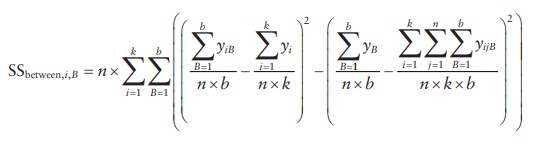
Calculations

The calculations for a two-way ANOVA experiment are similar to the one-way ANOVA, with the inclusion of the case of a second variable B at levels 1 through b. The equations for the one-way ANOVA in the corre-sponding previous section are considered as the effect of variable A. The equations are modified as below for inclusion of the effect of variable B.

1. Mean of all samples in the experiment (μ) is calculated by adding all observations and dividing by the total number of samples in the experiment.

where, y_ijk represents the jth observation of the ith level of treatment of the variable A and bth level of treatment of variable B, there being a total of k treatments (i = 1, 2, 3, … k) and n samples per treatment level (j = 1, 2, 3, …. n) for variable A and b treatments (B = 1, 2, 3, … b) and n samples per treatment level (j = 1, 2, 3, …. n) for variable B; N is the total sample size, including all treatments and levels.

2. Total sum of squares (SS_T) of all observations is calculated by squar-ing all observations and subtracting from the mean of all samples in the experiment (μ).

3. Sum of squares for the factor is the sum of squares between the col-umns (SS_between) if each level of the factor is arranged in a column. It is calculated by subtracting the mean value for each column from the mean of all samples, squaring this value, and adding for all columns.

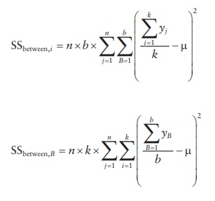
Sum of squares for interaction between factors A and B is determined by:

4. Sum of squares for the random error (SS_error) is the difference between the total sum of squares and the sum of squares between and within the columns.

SS_error = SS_total − SS_between,i − SS_between,B

5. Degrees of freedom are calculated as follows:

Degrees of freedom between groups (DF_between):

DF_between,i = k − 1

DF_between,B = b − 1

Degrees of freedom for the error term (DF_error):

DF_error = N − k × b

Degrees of freedom for the interaction term (DF_interaction):

DF_interaction = (k − 1)(b − 1)

6. Mean squares for the random error (MS_error) and the factor studied (MS_between) are calculated by dividing their respective sum of squares by their degrees of freedom.

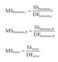
7. An F-ratio is computed as the ratio of mean squares of factor effect to the mean square of error effect.

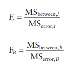
8. Determine critical F-ratio at (DF_between and DF_error) degrees of freedom for α = 0.05.

9. Test the hypothesis: The F-ratio is compared to the P_α value for the F-test at designated degrees of freedom to determine the significance of observed results. Statistical significance of results would indicate that the contribution of the factor’s or variable’s effect on the observa-tions is significantly greater than the variation that can be ascribed to random error.

Calculations using Microsoft Excel

As an illustration of two-way ANOVA calculations using Microsoft Excel’s data analysis add-in tool, the example summarized in Table 5.11 provides a tabular output of calculated values listed in Table 5.12.

Table 5.11 A hypothetical example of a two-way ANOVA experiment. Yield of a chemical synthesis reaction was studied as a function of temperature and pressure in a 2² full-factorial study without replication. The data, in terms of percentage yield, are summarized in the table

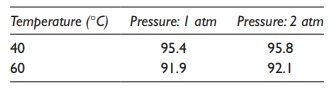
Table 5.12 Statistical results for a hypothetical example of a two-way ANOVA experiment using Microsoft Excel

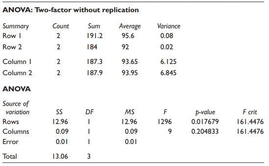
This tabular output of results summarizes statistical parameters asso-ciated with the data, followed by a summary of calculated results in a tabular format. The critical F-value and the p-value associated with the calculated F-value are indicated to facilitate hypothesis testing. Two-way ANOVA results provide information about statistical significance of differ-ences attributable to both factors. Thus, in this example, the contribution  of columns (pressure) to variation has a p-value of 0.20, while the contribu-tion of rows (temperature) has a p-value of 0.02. Given the α value of 0.05, the contribution of temperature is significant, while that of pressure is not.