Survival Probabilities: Life Tables

Survival Probabilities

Life Tables

Life tables give estimates for survival during time intervals and present the cumulative survival probability at the end of the interval. The key idea for estimating the cumulative survival for both life tables and the Kaplan–Meier curve is represented by the following result for conditional probabilities: Let t₂ > t₁. Let P(t₂|t₁) = P(X > t₂|X > t₁), where X = survival time, t₁ = time at the beginning of the interval, and t₂ = the time at the end of the interval. That is, P(t₂|t₁) is the conditional probability that a patient’s survival time X is at least t₂, given that we have observed the patient sur-viving to t₁. Using this conditional probability, we have the following product rela-tionship for a survival curve, S(t), as shown by Equation 15.1:

S(t₂) = P(t₂|t₁) S(t₁)        for any t₂ > t₁ ≥ 0 (15.1)

where

S = survival time

t₁ = initial time

t₂ = latter time point

For the life table, the key is to use the data in Table 15.1 to estimate P(t₂|t₁) at the endpoints of the selected intervals. Remember that S(t) denotes the survival function. For the first interval from [0, a], we know that for all patients S(0) = 1 and, accordingly, S(a) = P(a|0); i.e., all patients are alive at the beginning of the interval and a portion of them survive until time a.

The life table method, also referred to as the Cutler–Ederer method (Cutler and Ederer, 1958), is called an actuarial method because it is the method most often used by actuaries to establish premiums for insuring customers.

Now we will construct a life table for the data in Table 15.1. We note from the last column that the survival times, including the censored times, range from 1.5 months to 17.6 months. We will group the data in three-month intervals giving us seven intervals, namely, [0, 3), [3, 6), [6, 9), [9, 12), [12, 15), [15, 18), and [18, `). (See Table 15.2.) For each interval, we need to determine the number of subjects who died during that interval, the number withdrawn during the interval, the total number at risk at the beginning of the interval, and the average number at risk dur-ing the interval. From these quantities, we compute: (1) the estimated proportion who died during the interval, given that they survived the previous intervals; and (2) the estimated proportion who would survive during the interval given that they sur-vived during the previous intervals.

Table 15.2 uses eight terms that may be unfamiliar to the reader. Following are the precise definitions of these eight elements for a life table:

·        The first column is labeled “Time Interval.” We denote the jth interval I_j.

·        The number who die during the jth interval is D_j. (D_j counts all of the patients whose time of death occurs during the jth interval.)

·        The number withdrawn during the jth interval is W_j. (W_j counts all of the pa-tients whose censoring time occurs during the jth interval.)

·        The number at risk at the start of the jth interval is N_j. (This is the number of subjects who entered into the study minus all deaths and all withdrawals that occurred prior to the jth interval.)

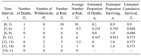
·        The average number at risk in the jth interval N_j’ = N_j –W_j/2. Referring to the second row of Table 15.2 under column N_j’, N_j’ = N_j – W_j/2 = 9 – ½ = 8.5. The term N_j’ reflects an actuarial technique to account for the fact that W_j of the patients who were at risk at the beginning of the interval are no longer at risk at the end of the interval.

·        N_j’ represents the average number of patients at risk in the interval when the withdrawals occur uniformly over the interval. We use N_j’ to improve the esti-mate of the probability of not surviving during the jth interval. We define q_j = D_j/N_j’ and assert that D_j/N_j’ is better than using D_j/N_j or D_j/N_j+1, where N_j+1 is the number at risk at the start of the j + 1 interval. We then define the estimate of the conditional probability of surviving during the interval given that the pa-tient survived during the previous j – 1 intervals as p_j. The estimate for surviv-ing past the jth interval is obtained by using the conditioning principle given in Equation 15.1. In Table 15.2 (second row), q_j = D_j/N_j’ = 2/8.5 = 0.235.

·        The estimated proportion surviving during the interval is p_j. From Table 15.2 (second row), p_j = (N_j’ – D_j)/N_j’ = [(8.5 –2)/8.5] = 0.765.

·        The cumulative survival estimate for the jth interval is denoted S_j and is de-fined recursively by S_j = p_j S_j–1.

The method of recursion allows one to calculate a quantity such as S_n by first calculating S₀ and then providing a formula that shows how to calculate S₁ from S₀. This same formula then can be used to calculate S₂ from S₁ and then S₃ from S₂ and so on until we get S_n from S_n–1. In the method of recursion, the equation is called a recursive equation. A calculation example will be given in the next section. Refer to Table 15.2 to see the terms that we defined in the list above.

TABLE 15.2. Life Table for Survival Times for Patients Using Data from Table 15.1 (N = 38)