Permutation Tests

PERMUTATION TESTS

Introducing Permutation Methods

The ranking procedures described in the present chapter have an advantage over parametric methods in that they do not depend on the underlying distributions of parent populations. As we will discuss in Section 14.9, ranking procedures are not sensitive to one or a few outlying observations. However, a disadvantage of ranking procedures is that they are less informative than corresponding parametric tests. In-formation is lost as a result of the rank transformations. For the sake of constructing a distribution-free method, we ignore the numerical values and hence the magnitude of differences among the observations. Note that if we observed the values 4, 5, and 6 we would assign them ranks 1, 2, and 3 respectively. On the other hand, had we observed the values 4, 5, and 10, we would still assign the ranks 1, 2, and 3, respec-tively. The fact that 10 is much larger than 6 is lost in the rankings.

Is there a way for us to have our cake and eat it too? Permutation tests retain the information in the numerical data but do not depend on parametric assumptions. They are computer-intensive techniques with many of the same virtues as the boot-strap.

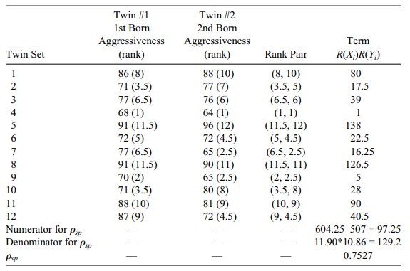
TABLE 14.12. Aggressiveness Scores for 12 Identical Twins

In the late 1940s and early 1950s, research confirmed that under certain condi-tions, permutation methods can be nearly as powerful as the most powerful para-metric tests. This observation is true as sample sizes become large [see, for exam-ple, Lehmann and Stein (1949) and Hoeffding (1952)]. Although permutation tests have existed for more than 60 years, their common usage has emerged only in the 1980s and 1990s. Late in the twentieth century, high-speed computing enabled one to determine the exact distributions of permutations under the null hypothesis. Per-mutation statistics generally have discrete distributions. Computation of all possible values of these statistics and their associated probabilities when the null hypothesis is true allows one to calculate critical values and p-values; the resulting tables are much like normal probability tables used for parametric Gaussian distributions

The concepts underlying permutation tests, also called randomization tests, go back to Fisher (1935). In the case of two populations, assume we have data from two distributions denoted as X₁, X₂, . . . , X_n for the first population, and Y₁, Y₂, . . . , Y_m for the second population. The test statistic is T = ΣX_i; we ask the question “How likely is it that we would observe the value T that we obtained if the Xs and the Ys really are independent samples from the same distribution?” This is our “null hy-pothesis”: the two distributions are identical and the samples are obtained indepen-dently.

The first assumption for this test is that both samples are independent random samples from their respective parent populations. The second is that at least an in-terval measurement scale is being used. Under these conditions, and assuming the null hypothesis to be true, it makes sense to pool the data because each X and Y gives information about the common distribution for the two samples.

As it makes no difference whether we include an X or a Y in the calculation of T, any arrangement of the n + m observations that assigns n to group one and m to group two is as probable as the other. Hence, under the null hypothesis, any assign-ment to the Xs of n out of the n + m observations constitutes a value for T. Recall from Chapter 5 that there are exactly C(n + m, n) = (n + m)!/[n! m!] ways to select n observations from pooled data to serve as the Xs.

Each arrangement leads to a potentially different value for T (some arrangements may give the same numerical values if the Xs and Ys are not all different values). The test is called a permutation test because we can think of the pooled observations as Z₁, Z₂, . . . , Z_n, Z_n+1, Z_n+2, . . . , Z_n+m, where the first n of Zs are the original Xs and the next m are the Ys. The other combinations can be obtained by a permutation of the indices from 1 to n + m, where the Xs are taken to be the first n indices after the permutation.

The other name for a permutation test—randomization test—comes about be-cause each selection of ns assigned to the Xs can be viewed as a random selection of n of the samples. This condition applies when the samples are selected at random out of the set of n + m values. Physically, we could mark each of the n + m values on a piece of paper, place and mix them in a hat and then reach in and randomly draw out n of them without replacing any in the hat. Hence, permutation methods also are said to be sampling without replacement. Contrast this to a bootstrap sample that is se-lected by sampling a fixed number of times but always with replacement.

Since under the null hypothesis each permutation has the probability 1/C(n + m, n), in principle we have the null distribution. On the other hand, if the two popula-tions really are different, than the observed T should be unusually low if the Xs tend to be smaller than the Ys and unusually large if the Xs tend to be larger than the Ys. The p-value for the test is then the sum of the probabilities for all permutations leading to values of T as extreme or more extreme (equal or larger or smaller) than the observed T.

So if k is the number of values as extreme as or more extreme than the observed T, the p-value is k/C(n + m, n). Such a p-value can be one-sided or two-sided depending on how we define “more extreme.” The process of determining the distribution of the test statistic (T) is in principle a very simple procedure. The problem is that we must enumerate all of these permutations and calculate T for each one to construct the cor-responding permutation distribution. As n and m become large, the process of gener-ating all of these permutations is a very computer-intensive procedure.

The basic idea of enumerating a multitude of permutations has been generalized to many other statistical problems. The problems are more complicated but the idea remains the same, namely, that a permutation distribution for the test can be calcu-lated under the null hypothesis. The null distribution will not depend on the shape of the population distributions for the original observations or their scores.

Several excellent texts specialize in permutation tests. See, for example, Good (2000), Edgington (1995), Mielke and Berry (2001), or Manly (1997). Some books with the word “resampling” in the title include permutation methods and comparethem with the bootstrap. These include Westfall and Young (1993), Lunneborg (2000), and Good (2001).

Another name for permutation tests is exact tests. The latter term is used be-cause, conditioned on the observed data, the significance levels that are determined for the hypothesis test have a special characteristic: The significance levels satisfy the exactness property regardless of the population distribution of the pooled data.

In the 2 × 2 contingency table in Section 11.6, we considered an approximate chi-square test for independence. The next section will introduce an exact permuta-tion test known as Fisher’s exact test. This test can be used in a 2 × 2 table when the chi-square approximation is not very good.

Fisher’s Exact Test

In a 2 × 2 contingency table, the elements are sometimes all random, but there are occasions when the row totals and the column totals are restricted in advance. In such cases, a permutation test for independence (or differences in group propor-tions), known as Fisher’s exact test, is appropriate. The test is attributed to R. A. Fisher, who describes it in his design of experiments text (Fisher, 1935). However, as Conover (1999) points out, it was also discovered and presented in the literature almost simultaneously in Irwin (1935) and Yates (1934).

Fisher and others have argued for its more general use based on conditioning ar-guments. As Conover (1999) points out, it is very popular for all types of 2 × 2 ta-bles because its exact p-values can be determined easily (by enumerating all the more extreme tables and their probabilities under the null hypothesis). As in the chapter on contingency tables, the null hypothesis is that if the rows represent two groups, then the proportions in the first column should be the same for each group (and, consequently, so should the proportions in the second column).

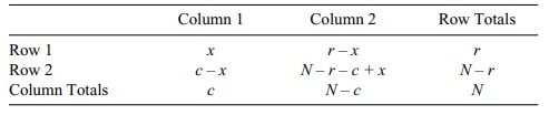
Consider N observations summarized in a 2 × 2 table. The row totals r and N – r and the column totals c and N – c are fixed in advance (or conditioned on after-wards). Refer to Table 14.13.

Because the values of r, c, and N are fixed in advance, the only quantity that is ran-dom is x, the entry in the cell corresponding to the intersection of Row 1 and Column 1. Now, x can vary from 0 up to the minimum of c and r. This limit on the value is due to the requirement that the row and column totals must always be r for the first row and c for the first column. Each different value of x determines a new distinct contin-gency table. Let us specify the null hypothesis that the probability p₁ of an observa-tion in row 1, column 1 is the same as the probability p₂ of an observation in row 2, column 1. The null distribution for the test statistic T, defined to be equal to x, is the hypergeometric distribution. Equation 14.9 defines the test statistic T.

TABLE 14.13. Basic 2 × 2 Contingency Table for Fisher’s Exact Test

While not covered explicitly in previous chapters, the hypergeometric distribu-tion is similar to discrete distributions that were discussed in Chapter 5. Remember that a discrete distribution is defined on a finite set of numbers. The hypergeometric distribution used for calculating test statistic for Fisher’s exact test is given in Equa-tion 14.9. Let T be the cell value for column 1, row 1 in a 2 × 2 contingency table with the constraints that the row one total is r and the column one total is c, with r and c less than or equal to the grand total N. Then for x = 0, 1, . . . , min(r, c),

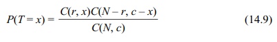
and P(T = x) = 0 for all other values of x.

A one-sided p-value for Fisher’s exact test is calculated as follows:

1. Find all 2 × 2 tables with the row and column totals of the observed table and with row 1, column 1 cell values equal to or smaller than the observed x.

2. Use the hypergeometric distribution from Equation 14.9 to calculate the probability of occurrence of these tables under the null hypothesis.

3. Sum the probabilities over all such tables.

The result at step (3) is the one-sided p-value. Two-sided and opposite one-sided p-values can be obtained according to a similar procedure. One needs to define the re-jection region such that it is the area on one tail of the distribution that is comprised of probabilities that are as extreme as or more extreme than the significance level of the test. The second side or the opposite side would be the corresponding area on the opposite end of the distribution. The next example will illustrate how to carry out the procedure described above.

Example: Lady Tasting Tea

Fisher (1935) gave a now famous example of a lady who claims that she can tell sim-ply by tasting tea whether milk or tea was poured into a cup first. Fisher used this ex-ample to demonstrate the principles of experimental design and hypothesis testing.

Let us suppose, as is described in Agresti (1990), page 61, that an experiment was conducted to test whether the lady simply is taking guesses versus the alterna-tive that she has the skill to determine the order of pouring the two liquids. The lady is given eight cups of tea, four with milk poured first and four with tea poured first. The cups are numbered 1 to 8. The experimenter has recorded on a piece of paper which cup numbers had the tea poured first and which had the milk poured first.

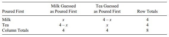
The lady is told that four cups had milk poured first and four had tea poured first. Given this information, she will designate four of them for each group. This design is important because it forces each row and column total to be fixed (see Table 14.14). 

TABLE 14.14. Lady Tasting Tea Experiment: 2 × 2 Contingency Table for Fisher’s Exact Test

In this experiment, the use of Fisher’s exact test is appropriate and uncon-troversial. For other designs, the application of Fisher’s exact test may be debatable even when there are some similarities to the foregoing example.

For this problem, there are only five contingency tables: (1) Correctly labeling all four cups with milk poured first and, hence, all with tea poured first; (2) incorrectly labeling one with milk poured first and, hence, one with tea poured first; (3) incor-rectly labeling two with milk poured first (also two with tea poured first); (4) incor-rectly labeling three with milk poured first (also three with tea poured first); and (5) incorrectly labeling all four with milk poured first (also all four with tea poured first).

Case (3) is the most likely under the null hypothesis, as it would be expected from random guessing. Cases (1) and (2) favor some ability to discriminate, and (4) and (5) indicate good discrimination but in the wrong direction. However, the sam-ple size is too small for the test to provide very strong evidence for the lady’s abili-ties, even in the most extreme cases in this example when she guesses three or four outcomes correctly.

Let us first compute the p-value when x is 3. In this case, it is appropriate to per-form a one-sided test, as a significant test statistic would support the claim that she can distinguish the order of pouring milk and tea. We are testing the alternative hy-pothesis that the lady can determine that the milk was poured before the tea versus the null hypothesis that she cannot tell the difference in the order of pouring. Thus, we must evaluate two contingency tables, one for x = 3 and one for x = 4. The ob-served data are given in Table 14.15.

The probability associated with the observed table under the null hypothesis is C(4, 3) C(4, 1)/C(8, 4) = (4 4 4!)/(8 7 6 5) = 8/35 = 0.229. The only table more ex-treme that favors the alternative hypothesis is the perfect table, Table 14.16.

TABLE 14.15. Lady Tasting Tea Experiment: Observed 2 × 2 Contingency Table for Fisher’s Exact Test

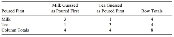
TABLE 14.16. Lady Tasting Tea Experiment: More Extreme 2 × 2 Contingency Table for Fisher’s Exact Test

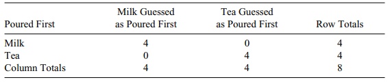
The probability of this table under the null hypothesis is 1/C(8, 4) = 1/ 70 = 0.0142. So the p-value for the combined tables is 0.229 + 0.014 = 0.243. If we ran the tea drinking experiment and observed an x of 3, we would have an observed p-value of 0.243; this outcome would suggest that we cannot reject the null hypothe-sis that the lady is unable to discriminate between milk or tea poured first.