Exercises questions answers

EXERCISES

12.1 Give in your own words definitions of the following terms that pertain to bi-variate regression and correlation:

a.     Correlation versus association

b.     Correlation coefficient

c.      Regression

d.     Scatter diagram

e.      Slope (b)

12.2 Research papers in medical journals often cite variables that are correlated with one another.

a.     Using a health-related example, indicate what investigators mean when they say that variables are correlated.

b.     Give examples of variables in the medical field that are likely to be cor-related. Can you give examples of variables that are positively correlated and variables that are negatively correlated?

c.      What are some examples of medical variables that are not correlated? Provide a rationale for the lack of correlation among these variables.

d.     Give an example of two variables that are strongly related but have a correlation of zero (as measured by a Pearson correlation coefficient).

12.3 List the criteria that need to be met in order to apply correctly the formula for the Pearson correlation coefficient.

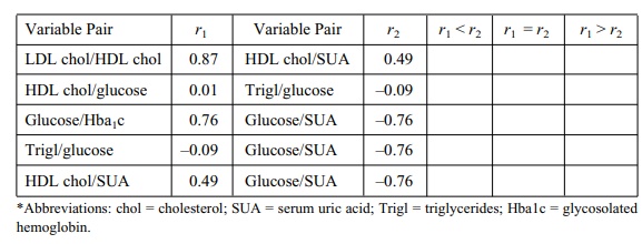
12.4 In a study of coronary heart disease risk factors, an occupational health physician collected blood samples and other data on 1000 employees in an industrial company. The correlations (all significant at the 0.05 level or higher) between variable pairs are shown in Table 12.12. By checking the appropriate box, indicate whether the correlation denoted by r₁ is lower than, equal to, or higher than the correlation denoted by r₂.

12.5 Some epidemiologic studies have reported a negative association between moderate consumption of red wine and coronary heart disease mortality. To what extent does this correlation represent a causal association? Can you identify any alternative arguments regarding the interpretation that consumption of red wine causes a reduction in coronary heart disease mortality?

TABLE 12.12. Correlations between Variable Pairs in a Risk Factor Study*

12.6 A psychiatric epidemiology study collected information on the anxiety and depression levels of 11 subjects. The results of the investigation are present-ed in Table 12.13. Perform the following calculations:

a.     Scatter diagram

b.     Pearson correlation coefficient

c.      Test the significance of the correlation coefficient at a = 0.05 and a = 0.01.

12.7 Refer to Table 12.1 in Section 12.3. Calculate r between systolic and dias-tolic blood pressure. Calculate the regression equation between systolic and diastolic blood pressure. Is the relationship statistically significant at the 0.05 level?

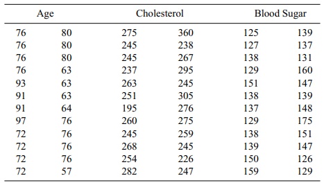
12.8 Refer to Table 12.14:

a.     Create a scatter diagram of the relationships between age (X) and choles-terol (Y), age (X) and blood sugar (Y), and cholesterol (X) and blood sug-ar (Y).

b.     Calculate the correlation coefficients (r) between age and cholesterol, age and blood sugar, and cholesterol and blood sugar. Evaluate the sig-nificance of the associations at the 0.05 level.

c.      Determine the linear regression equations between age (X) and choles-terol (Y), age (X) and blood sugar (Y), and cholesterol (X) and blood sug-ar (Y). For age 93, what are the estimated cholesterol and blood pressure values? What is the 95% confidence interval about these values? Are the slopes obtained for the regression equations statistically significant (at the 0.05 level)? Do these results agree with the significance of the correlations?

TABLE 12.13. Anxiety and Depression Scores of 11 Subjects

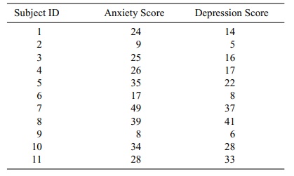
TABLE 12.14 : Age, Cholesterol Level, and Blood Sugar Level of Elderly Men

12.9 An experiment was conducted to study the effect on sleeping time of in-creasing the dosage of a certain barbiturate. Three readings were made at each of three dose levels:

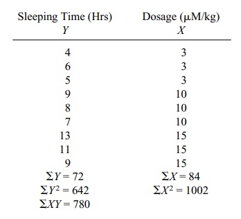
a.     Plot the scatter diagram.

b.     Determine the regression line relating dosage (X) to sleeping time (Y).

c.      Place a 95% confidence interval on the slope parameter β.

d.     Test at the 0.05 level the hypothesis of no linear relationship between the two variables.

e.      What is the predicted sleeping time for a dose of 12 μM/kg?

12.10 In the text, a correlation matrix was described. Using your own words, ex-plain what is meant by a correlation matrix. What values appear along the diagonal of a correlation? How do we account for these values?

12.11 An investigator studying the effects of stress on blood pressure subjected mine monkeys to increasing levels of electric shock as they attempted to obtain food from a feeder. At the end of a 2-minute stress period, blood pressure was measured. (Initially, the blood pressure readings of the nine monkeys were essentially the same).

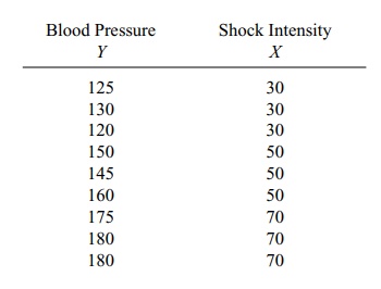
Some helpful intermediate calculations: ΣX = 450, ΣY = 1365, ΣX² = 24900, ΣY² = 211475, (ΣX)² = 202500, (ΣY)² = 1863225, ΣX Y = 71450, and (ΣX)( ΣY) = 614250. Using this information,

a.     Plot the scatter diagram.

b.     Determine the regression line relating blood pressure to intensity of shock.

c.      Place a 95% confidence interval on the slope parameter β.

d.     Test the null hypothesis of no linear relationship between blood pressure and shock intensity (stress level). (Use α = 0.01.)

e.      For a shock intensity level of 60, what is the predicted blood pressure?

12.12 Provide the following information regarding outliers.

a.     What is the definition of an outlier?

b.     Are outliers indicators of errors in the data?

c.      Can outliers sometimes be errors?

d.     Give an example of outliers that represent erroneous data.

e.      Give an example of outliers that are not errors.

12.13 What is logistic regression? How is it different from ordinary linear regres-sion? How is it similar to ordinary linear regression?

12.14 In a study on the elimination of a certain drug in man, the following data were recorded:

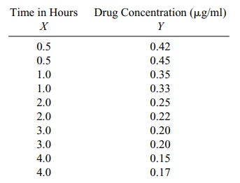
Intermediate calculations show ΣX = 21, ΣY = 2.74, ΣX² = 60.5, ΣY² = 0.8526, and ΣX Y = 4.535.

a.     Plot the scatter diagram.

b.     Determine the regression line relating time (X) to concentration of drug (Y).

c.      Determine a 99% confidence interval for the slope parameter β.

d.     Test the null hypothesis of no relationship between the variables at α = 0.01.

e.      Is (d) the same as testing that the slope is zero?

f.       Is (d) the same as testing that the correlation is zero?

g.     What is the predicted drug concentration after two hours?

12.15 What is the difference between a simple and a multiple regression equation?

12.16 Give an example of a multiple regression problem and identify the terms in the equation.

12.17 How does the multiple correlation coefficient R² for the sample help us in-terpret a multiple regression problem?

12.18 A regression problem with five predictor variables results in an R² value of 0.75. Interpret the finding.

12.19 When one of the five predictor variables in the preceding example is elimi-nated from the analysis, the value of R² drops from 0.75 to 0.71. What does this tell us about the variable that was dropped?

12.20 What is multicollinearity? Why does it occur in multiple regression problems?

12.21 What is stepwise regression? Why is it used?

12.22 Discuss the regression toward the mean phenomenon. Give a simple real-life example.

12.23 Give an example of a logistic regression problem. How is logistic regres-sion different from multiple linear regression?

12.24 When a regression model is nonlinear or the error terms are not normally distributed, the standard hypothesis testing methods and confidence inter-vals do not apply. However, it is possible to solve the problem by bootstrap-ping. How might you bootstrap the data in a regression model? [Hint: There are two ways that have been tried. Consider the equation Y = α + β₁X₁ + β₂X₂ + β₃X₃ + β₄X₄ + ε and think about using the vector (Y, X₁, X₂, X₃, X₄). Alternatively, to help you apply the bootstrap, what do you know about the properties of ε and its relationship to the estimated residuals e = Y – (a + b₁X₁ + b₂X₂ + b₃X₃ + b₄X₄), where a, b₁, b₂, b₃, and b₄ are the least squares estimates of the parameters α, β₁, β₂, β₃, and β₄, respectively.] Refer to Table 12.1 in Section 12.3. Calculate r between systolic and diastolic blood pressure. Calculate the regression equation between systolic and diastolic blood pressure. Is the relationship statistically significant at the 0.05 level?

Answers:

12.3 We assume that X and Y have a bivariate normal distribution. Then the re-gression E(Y|X) is linear. Then the product moment correlation has an interpreta-tion as a parameter of the bivariate normal distribution that represents the strength of the linear relationship. Even if X and Y do not have the bivariate normal distri-bution, if we can assume that Y = α + βx + ε, where ε is a random variance with mean 0 and variance σ² independent of X, then the sample product moment cor-relation is still a measure of the strength of the linear relationship between X and Y.

12.7 The scatter plot and the regression line are given in the following figure:

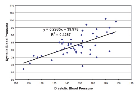
Systolic blood pressure versus diastolic blood pressure.

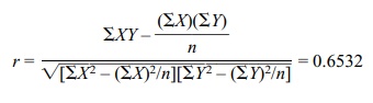
r = √0.4267 = 0.6532. Recall that [b – T_1–a/2SE(b), b + T_1–a/2SE(b)] where is the 100(1 – α /2) percentile for Student’s t distribution with n – 2 degrees of freedom. This interval is a 100(1 – α)% confidence interval for β. Here we require α to be 0.05. So T_1–a/2 = 1.679 since the degrees of freedom equals 46. To get SE(b) recall that SSE = Σ(y – Yˆ)², S_y.x = √SSE/n – 2, and SE(b) = S_y.x/ √Σ(x – ). Now SSE = 1516.30, so SSE/(n – 2) = 1516.30/46 = 32.96. So S_y.x = 5.7413 and √Σ(x – )² = 114.4595. So SE(b) = 5.7413/114.4595 = 0.05016. Hence the confidence interval is [b – T_1–a/2SE(b), b + T_1–a/2SE(b)] = [0.2935 – 1.679(0.05016), 0.2935 + 1.679(0.05016)] = [0.2093, 0.3777]. Recall that testing the significance of a linear relationship is the same as testing that the slope parameter is zero, which in turn is equivalent to testing whether the correlation r is zero. 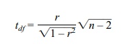Recall the t test as follows:

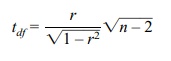
where df = n – 2 and n = number of pairs. Here n = 48 and

So t = 0.6532√46/ √(1 – 0.4267) = 4.4302/0.75717 = 5.851 Comparing this to a t with 46 degrees of freedom we find the critical T at the 5% level (two-sided) is 1.679, Since 5.475 is larger than 1.679, we reject the null hypothesis.

12.9 The scatter plot and the regression line are given in the following figure:

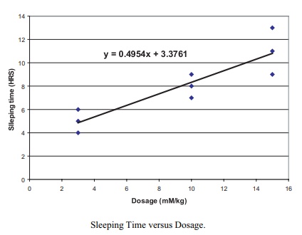
Sleeping Time versus Dosage.

b. y = 0.4954x + 3.3761

c. Recall that [b – T_1–a/2SE(b), b + T_1–a/2SE(b)] where is the 100(1 – a/2) percentile for Student’s t distribution with n – 2 degrees of freedom. This interval is a 100(1 – α)% confidence interval for β. Here we require a to be 0.05. So T_1–a/2 =  2.3646 since the degrees of freedom equals 7. To get SE(b) recall that SSE = Σ(y –Y ˆ)², S_y.x = √(SSE/n – 2), and SE(b) = S_y.x/ √[Σ(x – )²]. Now SSE = 12.49541, so SSE/(n – 2) = 12.48541/7 = 1.78363. So S_y.x = 1.33553 and √[Σ(x – )²] = 14.7648. So SE(b) =  1.33553/14.7648 = 0.09045. Hence the confidence interval is [b – T_1–a/2SE(b), b + T_1–a/2SE(b)] = [0.4954 – 2.3646(0.09045), 0.4954 + 2.3646(0.09045)] = [0.2815, 0.7093].

d. Recall that testing the significance of a linear relationship is the same as test-ing that the slope parameter is zero, which in turn is equivalent to testing whether the correlation r is zero. Recall the t test as follows:

where df = n – 2 and n = number of pairs. Here n = 9 and r = ΣXY – (ΣX)( ΣY)/n/ √{[ΣX² – (ΣX)²/n][ ΣY² – (ΣY)²/n]} = {780 – (84)(72)/9}/{√1002 – (84)²/9√642 – (72)²/9} = 108/{ √218 √66} = 108/119.95 = 0.9004. So t = 0.9004 √7/ √(1 – 0.8107) = 5.475. Comparing this to a t with 7 degrees of freedom, we find the critical T at the 5% level (two-sided) is 2.3646. Since 5.475 is larger than 2.3646, we reject the null hypothesis.

e. y = 0.4954(12) + 3.3761 = 9.3209.

12.17 The sample multiple correlation coefficient R² in a multiple regression problem represents the percentage of the variation in Y that is explained by the pre-dictor variables through the linear regression equation. A value of 1 indicates a per-fect linear fit to the data. A value close to 1 indicates a good fit.

12.18 The drop in R² from 0.75 to 0.71 indicates that the addition of the fifth vari-able only explains an additional 4% of the variance in Y. This may not be explaining enough of the variation to include this variable in the model. Depending on the sam-ple size this may or may not be statistically significant

12.21 Stepwise regression is a method for added and deleting variables in a step-wise fashion based on which variable in the equation is weakest and which from the list of possible entrants is strongest based on criteria such as “F to enter” and “F to exit.” It is used to help pick a good subset of the variables for inclusion in the model.

12.23 An example of a logistic regression problem would be the military triage problem. In the case where a soldier is wounded and is in shock, the chances of his survival depends on the severity of his injury, which can be determined by several measurements including blood pressure. The army may in combat be faced with too many severely wounded soldiers to be able to treat all of them. When having to choose which patients to treat, the army wants to know the chance of survival. A lo-gistic regression equation can predict the chance of survival of a patient based on vital signs. The equation can be developed based on historical data for shock trauma patients. In logistic regression, the outcome variable Y is binary. The patient sur-vives or dies. A logit transformation is applied to the response before creating a lin-ear relationship with the predictors. Ordinary least squares is no longer available as a simple analytic method for obtaining the regression parameters. The predictor variables can be continuous or discrete as in an ordinary multiple regression equa-tion. Because the outcome variable is binary, its expected value is a proportion that represents the probability of the outcome associated with the value 1.