Exercises questions answers
| Home | | Advanced Mathematics |Chapter: Biostatistics for the Health Sciences: Summary Statistics
Biostatistics for the Health Sciences: Summary Statistics - Exercises questions answers
EXERCISES
4.1 What is meant by a measure of location? State in
your own words the defini-tions of the following measures of location:
a. Arithmetic mean
b. Median
c. Mode
d. Uni-, bi-, and multimodal distributions
e. Skewed distributions—positively and negatively
f. Geometric mean
g. Harmonic mean
4.2 How are the mean, median, and mode interrelated?
What considerations lead to the choice of one of these measures of location
over another?
4.3 Why do statisticians need measures of variability?
State in your own words the definitions of the following measures of
variability:
a. Range
b. Mean absolute deviation
c. Standard deviation
4.4 How are the mean and variance of a distribution
affected when:
a. A constant is added to every value of a variable?
b. Every value of a variable is multiplied by a constant?
4.5 Giving appropriate examples, explain what is meant
by the following statement: “Sm2
is a biased or unbiased estimator of the parameter σ2.”
4.6 Distinguish among the following formulas for
variance:
a. Finite population variance
b. Sample variance (deviation score method)
c. Sample variance (deviation score method for grouped data)
d. Sample variance (calculation formula)
4.7 Define the following terms and indicate their
applications:
a. Coefficient of variation
b. Coefficient of dispersion
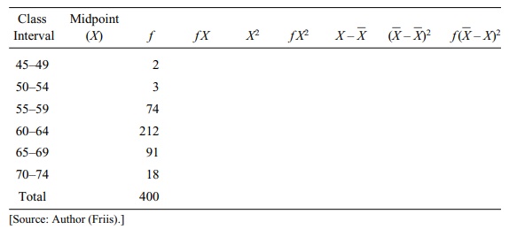
4.8 The table below frequency table showing heights in
inches of a sample of fe-male clinic patients. Complete the empty cells in the
table and calculate the sample variance by using the formula for grouped data.
4.9 Find the medians of the following data sets: {8,
7, 3, 5, 3}; {7, 8, 3, 6, 10, 10}.
4.10 Here is a dataset for mortality due to work-related
injuries among African American
women in the United States during 1997: {15–24 years (9); 25–34 years (12);
35–44 years (15); 45–54 years (7); 55–64 years (5)}.
a. Identify the modal class.
b. Calculate the estimated median.
c. Assume that the data are for a finite population and compute the
variance.
d. Assume the data are for a sample and compute the variance.
4.11 A sample of data was selected from a population:
{195, 179, 205, 213, 179, 216, 185, 211}.
a. Use the deviation score method and the calculation formula to calculate
variance and standard deviations.
b. How do the results for the two methods compare with one another? How
would you account for discrepancies between the results obtained?
4.12 Using the data from the previous exercise, repeat
the calculations by applying the
deviation score method; however, assume that the data are for a finite
population.
4.13 Assume you have the following datasets for a sample:
{3, 3, 3, 3, 3}; {5, 7, 9, 11}; {4,
7, 8}; {33, 49}
a. Compute S and S2.
b. Describe the results you obtained.
4.14 Here again are the seasonal home run totals for the
four baseball home run sluggers we
compared in Chapter 3:
McGwire 49, 32, 33, 39, 22, 42, 9, 9, 39, 52, 58, 70,
65, 32
Sosa 4, 15, 10, 8, 33, 25, 36, 40, 36, 66, 63, 50
Bonds 16, 25, 24, 19, 33, 25, 34, 46, 37, 33, 42,
40, 37, 34, 49
Griffey 16, 22, 22, 27, 45, 40, 17, 49, 56, 56, 48,
40
a. Calculate the sample average number of home runs per season for each
player.
b. Calculate the sample median of the home runs per season for each player.
c. Calculate the sample geometric mean for each player.
d. Calculate the sample harmonic mean for each player.
4.15 Again using the data for the four home run sluggers
in Exercise 4.14, calcu-late the following measures of dispersion:
a. Each player’s sample range
b. Each player’s sample standard deviation
c. Each player’s mean absolute deviation
4.16 For each baseball player in Exercise 4.14,
calculate their sample coefficient of
variation.
4.17 For each baseball player in Exercise 4.14,
calculate their sample coefficient of
dispersion.
4.18 Did any of the results in Exercise 4.17 come close
to 1.0? If one of the play-ers did have a coefficient of dispersion close to 1,
what would that suggest about the distribution of his home run counts over the
interval of a baseball season?
4.19 The following cholesterol levels of 10 people were
measured in mg/dl: {260,150, 165, 201, 212, 243, 219, 227, 210, 240}. For this
sample:
a. Calculate the mean and median.
b. Calculate the variance and standard deviation.
c. Calculate the coefficient of variation and the coefficient of
dispersion.
4.20 For the data in Exercise 4.19, add the value 931
and recalculate all the sample values
above.
4.21 Which statistics varied the most from Exercise 4.19
to Exercise 4.20? Which statistics
varied the least?
4.22 The eleventh observation of 931 is so different
from all the others in Exercise 4.19
that it seems suspicious. Such extreme values are called outliers. Which
estimate of location do you trust more when this observation is included, the
mean or the median?
4.23 Answer the following questions:
a. Can a population have a zero variance?
b. Can a population have a negative variance?
c. Can a sample have a zero variance?
d. Can a sample have a negative variance?
Answer:
4.1 Measures of location are statistical estimates that
describe the center of a probability
distribution. Some measures are more appropriate than others, depend-ing on the
shape of the distribution.
a. The arithmetic mean is the
“center of gravity” for the distribution. It is simply the sum of the
observations divided by the number of observations. It is an appro-priate
measure for symmetric distributions like the normal distribution.
b. The median is the middle
value. For an odd number of samples, that is, if n = 2m + 1, an odd
number, the median is the m + 1 value
when ordered from smallest to largest. If n
= 2m, an even number, then the median
is the average of the m and m + 1 values ordered from smallest to largest.
Approximately half the values are be-low and half are above the median.
c. The mode is the most frequently occurring value
(or values if more than one value tie for most frequent). For a density
function, the mode is the peak in the den-sity (i.e., the top of the mountain).
d. A unimodal distribution is one
that has a density with only one peak. A bi-modal distribution is one with a
density that has two peaks (not necessarily equal). Mutimodal distributions
have two or more peaks.
e. Skewed distributions are
distributions that are not symmetric. A right or posi-tively skewed
distribution has a long trailing tail to the right. A left or negatively skewed
distribution has the distribution concentrated to the right with the longer
tail to the left.
f. The geometric mean for a
sample of size n is the nth root of the product of the
observations. The log of the geometric mean is the arithmetic mean of the
loga-rithms. Cosnequently, the geometric mean is appropriate for the lognormal
distribu-tion and distribution with shape similar to the lognormal.
g. The harmonic mean of a sample
is the reciprocal of average of the reciprocal of the observations.
4.9 The first data set is odd since it contains 5
values {8, 7, 3, 5, 3}. Ordering the data
from smallest to largest, we get the sequence 3, 3, 5, 7, 8. The third
observation in this sequence is the median. Hence, the median is 5. The second
data set is even since it contains 6 values {7, 8, 3, 6, 10, 10}. Ordering them
from smallest to largest we get 3, 6, 7, 8, 10, 10. In this sequence, the third
observation is the one just below the middle and the fourth is the observation
just above. So by the definition of sam-ple median, the median is the average
of these observations (7 + 8)/2 = 7.5.
4.13 a. First the sample mean is calculated as (3 + 3 +
3 + 3 + 3)/5 = 3. Next calcu-late the squared deviations (3 – 3)2 =
0, (3 – 3)2 = 0, (3 – 3)2 = 0, (3 – 3)2 = 0,
and (3 - 3)2 = 0. Add up the terms and divide by n – 1 = 4 to get 0 for S2. The sample stan-dard
deviation is the square root of the answer is √0 = 0.
The shortcut formula is
S2 = { Σx2i – nm2 } / (n – 1)
where m
is the sample mean and n is the
sample size. Σx2i = 32 + 32 + 32 +
32 + 32 = 45. nm2
= 5(3)2 = 45. So S2
= (45 – 45)/4 = 0.
In the second case, the sample mean is (5 + 7 + 9 +
11)/4 = 32/4 = 8. Next calcu-late the squared deviations (5 – 8)2 =
9, (7 – 8)2 = 1, (9 – 8)2 = 1, and (11 – 8)2 =
9. Add up the terms and divide by n –
1 = 3 to get 20/3 = 6.67 for S2.
The sample stan-dard deviation is the square root of the answer is √6.67 = 2.58. The shortcut formula is
S2 = { Σx2i – nm2 } / (n – 1)
where m
is the sample mean and n is the
sample size. Σx2i = 52 + 72 + 92 +
112 = 276. nm2
= 4(8)2 = 256. So S2
= (276 – 256)/3 = 20/3 = 6.67.
In the last example, we have just 2 observations,
33 and 49. The mean is 41. Next calculate the squared deviations (33 – 41)2
= 64 and (4 9– 41)2 = 64. Add up the terms and divide by n – 1 = 1 to get 128 for S 2. The sample standard
deviation is the square root of the answer, √128 =
11.31. The shortcut formula is
S2 = { Σx2i – nm2 } / (n – 1)
where m
is the sample mean and n is the
sample size. Σx2i = 332 + 492 = 3490. nm2 = 2(41)2 = 3362. So S2 = (3490 – 3362)/1 = 128.
b. For the first sample, all the values were the
same. So there is no variation and the variance is zero.
4.15 In this problem, we use the home run sluggers data
to compare some mea-sures of dispersion. Recall that the data are as follows:
McGwire: 49, 32, 33, 39, 22, 42, 9, 9, 39, 52, 58, 70,
65, 32
Sosa 4, 15, 10, 8, 33, 25, 36, 40, 36, 66, 63, 50
Bonds 16, 25, 24, 19, 33, 25, 34, 46, 37, 33, 42,
40, 37, 34, 49
Griffey 16, 22, 22, 27, 45, 40, 17, 49, 56, 56, 48,
40
a. The sample ranges are 70 – 9 =
61 for McGwire, 66 – 4 = 62 for Sosa, 49 – 16 = 33 for Bonds, and 56 – 16 = 40
for Griffey.
b. We use the shortcut formula to calculate the
standard deviations. Recall that
S2 = { Σx2i – nm2 } / (n – 1)
For McGwire, the Σx2i = (49)2 + (32)2 + (33)2 + (39)2
+ (22)2 + (42)2 + (9)2 + (9)2 +
(39)2 + (52)2 + (58)2 + (70)2 +
(65)2 + (32)2 = 2401 + 1024 + 1089 + 1521 + 484 + 1764 +
81 + 81 + 1521 + 2704 + 3364 + 4900 + 4225 + 1024 = 26183, and since m = (49+32+33+39+22+42+9+9+39+52+58+70+65+32)/14=551/14
= 39.357, nm2 = 14(39.357)2
= 21685.786. So S2 =
(26183 – 21685.786)/13 = 345.94 and S
= √345.94 = 18.6.
For Sosa, the Σx2i = (4)2 + (15)2 + (10)2 + (8)2
+ (33)2 + (25)2 + (36)2 + (40)2 +
(36)2 + (66)2 + (63)2 + (50)2 = 16
+ 225 + 100 + 64 + 1089 + 625 + 1296 + 4356 + 3969 + 2500 = 14240, and since m = (4 + 15 + 10 + 8 + 33 + 25 + 36 + 40
+ 36 + 66 + 63 + 50)/12 = 386/12 = 32.167, nm2
= 12(32.167)2 = 12416.333. So S
2 = (14240 – 12416.333)/11 = 165.79 and S = √165.79 = 12.9.
For Bonds, the Σx2i = (16)2 + (25)2 + (24)2 + (19)2
+ (33)2 + (25)2 + (34)2 + (46)2 +
(37)2 + (33)2 + (42)2 + (40)2 +
(37)2 + (34)2 + (49)2 = 256 + 625 + 576 + 361
+ 1089 + 625 + 1156 + 2116 + 1369 + 1089 + 1764 + 1600 + 1369 + 1156 + 2401 =
17552, and since m = (16 + 25 + 24 +
19 + 33 + 25 + 34 + 46 + 37 + 33 + 42 + 40 + 37 + 34 + 49)/15 = 494/15 =
32.933, nm2 = 15(32.933)2
= 16269.0667. So S 2 =
(17552 – 16269.0667)/14 = 91.64 and S
= √91.64 = 9.57.
Finally, for Griffey, the Σx2i = (16)2 + (22)2 + (22)2
+ (27)2 + (45)2 + (40)2 + (17)2 +
(49)2 + (56)2 + (56)2 + (48)2 +
(40)2 = 256 + 484 + 484 + 729 + 2025 + 1600 + 289 + 2401 + 3136 +
3136 + 2304 + 1600 = 18444, and since m
= (16 + 22 + 22 + 27 + 45 + 40 + 17 + 49 + 56 + 56 + 48 + 40)/12 = 438/12 =
36.5, nm2 = 12(36.5)2
= 15987. So S 2 = (18444 –
15987)/11 = 223.36 and S = √223.36 = 14.95.
c. For McGwire, since m = 39.357, the sum of absolute deviations is |49 – 39.357| + |32 –
39.357| + |33 – 39.357| + |39 – 39.357| + |22 – 39.357| + |42 – 39.357| + |9 –
39.357| + |9 – 39.357| + |39 – 39.357| + |52 – 39.357| + |58 – 39.357| + |70 –
39.357| + |65 – 39.357| + |32 – 39.357| = 9.643 + 7.357 + 6.357 + 0.357 +
17.357 + 2.643 + 30.357 + 30.357 + 0.357 + 12.643 + 18.643 + 30.643 + 25.643 +
7.357 = 169.357. Divide by the sample size n
= 14 to get 12.097 for the sample mean absolute deviation.
Now, for Sosa, since m = 32.167, the sum of absolute deviations is |4 – 32.167| + |15 –
32.167| + |10 – 32.167| + |8 – 32.167| + |33 – 32.167| + |25 – 32.167| + |36 –
32.167| + |40 – 32.167| + |36 – 32.167| + |66 – 32.167| + |63 – 32.167| + |50 –
32.167| = 28.167 + 17.167 + 22.167 + 24.167 + 0.833 + 7.167 + 3.833 + 7.833 +
3.833 + 33.833 + 30.833 + 17.833 = 197.667. Divide by the sample size n = 12 to get 16.472 for the sample mean
absolute deviation.
Now, for Bonds, since m = 32.167, the sum of absolute deviations is |16 – 32.933| + |25 –
32.933| + |24 – 32.933| + |19 – 32.933| + |33 – 32.933| + |25 – 32.933| + |34 –
32.933| + |46 – 32.933| + |37 – 32.933| + |33 – 32.933| + |42 – 32.933| + |40 –
32.933| + |37 – 32.933| + |34 – 32.933| + |49 – 32.933| = 16.933 + 7.933 +
8.933 + 13.933 + 0.067 + 7.933 + 1.067 + 13.067 + 4.067 + 0.067 + 9.067 + 4.067
+ 1.067 + 16.067 = 104.268. Divide by the sample size n = 14 to get 7.448 for the sample mean absolute deviation.
Now, for Griffey, since m = 36.5, the sum of absolute deviations is |16 – 36.5| + |22 –
36.5| + |22 – 36.5| + |27 – 36.5| + |45 – 36.5| + |40 – 36.5| + |17 – 36.5| +
|49 – 36.5| + |56 – 36.5| + |56 – 36.5| + |48 – 36.5| + |40 – 36.5| = 20.5 +
14.5 + 14.5 + 9.5 + 8.5 + 3.5 + 19.5 + 12.5 + 19.5 + 19.5 + 11.5 + 3.5 = 157.
Divide by the sample size n = 12 to
get 13.083 for the sample mean absolute deviation.
By all measures, we see apparent differences in
variability among these players, even though their home run averages tend to be
similar in the range from 32 to 40. Bonds seems to be the most consistent
(i.e., has the smallest variability based on all three measures). Oddly, this
might change when the 2001 season is added in since he hit a record 73 home
runs that year, which is 24 more than his previous high of 49 in the 2000
season.
Related Topics
