Confidence Intervals for Proportions

CONFIDENCE INTERVALS FOR PROPORTIONS

First we will consider a single proportion and the approximate intervals based on the normal distribution. If W is X/n, where X is a binomially distributed random variable with parameters n and p, then by the central limit theorem W is approximately normally distributed with mean p and variance p(1 – p)/n. Therefore, (W – p)/ √{p(1 – p)/n} has an approximately standard normal distribution.

Because p is unknown, we cannot normalize W by dividing W by p. Instead, we consider the quantity U = (W – p)/ √{W(1 – W)/n}. Since W is a consistent estimate of p, this quantity U converges to a standard normal random variable as the sample size n increases.

Therefore, we use the fact that if U were standard normal, then P[–1.96 ≤ U ≤ 1.96] = 0.95 or P[–1.96 ≤ (W – p)/ √{W(1 – W)/n} ≤ 1.96] = 0.95 or, after the usual algebraic manipulations, P[W – 1.96 √{W(1 – W)/n} ≤ p ≤ W + 1.96 √{W(1 – W)/n}]. So the random interval [W – 1.96 √{W(1 – W)/n}, W + 1.96 √{W(1 – W)/n]} is an approximate 95% confidence interval for a single proportion p.

[W – 1.96 √{W(1 – W)/n},

W + 1.96 √{W(1 – W)/n]}               (10.6)

where W = X/n and X is binomially distributed with parameters n and p. For other confidence levels, change 1.96 to the appropriate constant C from the standard nor-mal distribution.

As an example, suppose that we have 16 successes in 20 trials; X = 16 and n = 20. What would be an approximate 95% confidence interval for the population proportion of successes, p? From Equation 10.6, since W = 16/20 = 0.80, we have [0.80 - 1.96 √[0.8(0.2)/20], 0.80 + 1.96 √{0.8(0.2)/20}] = [0.80 – 0.1753, 0.80 + 0.1753] = [0.625, 0.975]. Later we will compare this interval to the exact interval obtained by the Clopper–Pearson method.

Now let us consider two independent estimates of proportions, W₁ = X₁/n₁ and W₂ = X₂/n₂, where X₁ is a binomial random variable with parameters p₁ and n₁ and X₂ is a binomial random variable with parameters p₂ and n₂. Then, Z = (W₁ – W₂) – (p₁ – p₂)/ √{[W₁(1 – W₁)/n₁ + W₂(1 – W₂)/n₂]} has an approximately standard normal distribution. Therefore, P[–1.96 ≤ Z ≤ 1.96] is approximately 0.95. After substitution and algebraic manipulations, we have P[(W₁ – W₂) - 1.96 √ {[W₁(1 – W₁)/n₁ + W₂(1 – W₂)/n₂]} ≤ (p₁ – p₂) ≤ [(W₁ – W₂) +1.96 √{[W₁(1 – W₁)/n₁ + W₂(1 – W₂)/n₂]}. The probability that p₁ – p₂ lies within this interval is approximately 0.95; hence, the random interval [(W₁ – W₂) – 1.96 √{[W₁(1 – W₁)/n₁ + W₂(1 – W₂)/n₂]}[(W₁ – W₂) + 1.96 √{[W₁(1 – W₁)/n₁ + W₂(1 – W₂)/n₂]} is an approximate 95% confidence interval for p₁ – p₂.

An approximate 95% confidence interval for the difference between two propor-tions p₁ – p₂ is

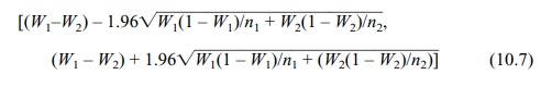
[(W₁–W₂) – 1.96 √{W₁(1 – W₁)/n₁ + W₂(1 – W₂)/n₂},

(W₁ – W₂) + 1.96 √{W₁(1 – W₁)/n₁ + (W₂(1 – W₂)/n₂)]}                     (10.7)

where W₁ = X₁/n₁ and X₁ is binomially distributed with parameters n₁ and p₁, and W₂ = X₂/n₂ and X₂ is binomially distributed with parameters n₂ and p₂. For other confidence levels, change 1.96 to the appropriate constant C from the standard nor-mal distribution.

For a numerical example, suppose n₁ is 100 and n₂ is 50. Suppose X₁ = 85 and X₂ = 26. We will calculate the approximate 95% and 99% confidence intervals for p₁ – p₂ when W₁ = 85/100 = 0.85 and W₂ = 26/50 = 0.52. In the case of the 95% confidence interval, the constant C = 1.96; hence, the interval is [(0.85 – 0.52) – 1.96 √{0.85(0.15)/100 + 0.52(0.48)/50}, (0.85–0.52)+1.96 √{0.85(0.15)/100 + 0.52(0.48)/50]} = [0.175, 0.485].

For exact intervals, the Clopper–Pearson method is used. Clopper and Pearson (1934) provided the results of their method in graphical form. Hahn and Meeker (1991) reprinted Clopper and Pearson’s work, along with much detail about confi-dence intervals. The two-sided interval uses the F distribution with the 100(1 – α)% interval given by Equation 10.8. We will learn about the F distribution in Chapter 13.

The exact 100(1 – a)% confidence interval for a single binomial proportion is

[{1 + (n – x + 1)F(1 – a/2:2n – 2x + 2, 2x)/x}^–1, {1 + (n – x)/{(x + 1)F(1 – a/2:2x + 2, 2n – 2x)}}^–1]

where x is the number of successes in n Bernoulli trials and F(γ: dfn, dfd) is the 100 γ th percentile of an F distribution with dfn degrees of freedom for the numerator and dfd degrees of freedom for the denominator. For the lower endpoint, γ = 1 – a/2, dfn = 2n – 2x, and dfd = 2x. For the upper endpoint, γ = 1 – α/2, dfn = 2x + 2, and dfd = 2n–2x.

Now let us revisit the example for approximate confidence intervals where X = 16, n = 20, and 1 – α/2 = 0.95. The above equation becomes [{1 + 5 F(0.95: 10, 32)/ 16}^–1, {1 + 4/{5 F(0.95: 34, 8)}}^–1]. For now we will take these percentiles by con-sulting a table for the F distribution. From the table (Appendix A), we see that F(0.95: 10, 32) = 2.94 and F(0.95: 34, 8) = 5.16 (by interpolation between F(0.95, 30, 8) = 5.20 and F(0.95, 40, 8) = 5.11. Plugging these values into Equation 10.8, we obtain the interval [0.521, 0.866]. The value 0.95 tells us the percentile to look up in the table; the two other parameters are the numerator and denominator de-grees of freedom, to be defined in Chapter 12.

Compare this new interval to the interval from the normal approximation [0.625, 0.975]. Note that the widths of the intervals are about the same, but the normal ap-proximation gives a symmetric interval centered at 0.80. The reason for the differ-ence is that the sample size of 20 is too small for the normal approximation to be very good, as the true proportion is probably close to 0.80; the Binomial distribu-tion, though centered at 0.80, is much more skewed than a normal distribution and has a longer left tail than right tail. In this case, the exact binomial solution is appro-priate but the normal approximation is not.

If n were 100, the normal approximation and the exact Binomial distribution would be in much closer agreement. So let us make the comparison when n = 100 and x = 80. The normal approximation gives [0.80–1.96 √{0.8(0.2)/100}, 0.80 + 1.96 √{0.8(0.2)/100}] = [0.722, 0.878], whereas the Clopper–Pearson method gives [{1 + 21 F(0.95: 42, 160)/80}^–1, {1 + 20/{81 F(0.95: 162, 40)}}^–1]. We have F(0.95: 42, = 1.72 (by interpolation in the table, Appendix A) and F(0.95: 162, 40) = 1.90 (also by interpolation in the table). Substituting these values in the equation above gives the interval [0.689, 0.885]. We note that the normal approximation, though not as accurate as we would like, is much closer to the exact result when the sample size is 100 as compared to when the sample size is only 20.