Bootstrap Percentile Method Confidence Intervals

BOOTSTRAP PERCENTILE METHOD CONFIDENCE INTERVALS

Now that you have learned the bootstrap principle, it is relatively simple to generate percentile method confidence intervals for the mean. The advantages of the bootstrap confidence interval are that (1) it does not rely on any parametric distributional assumptions; (2) there is no reliance on a central limit theorem; and (3) there are no complicated formulas to memorize. All you need to know is the boot-strap principle. 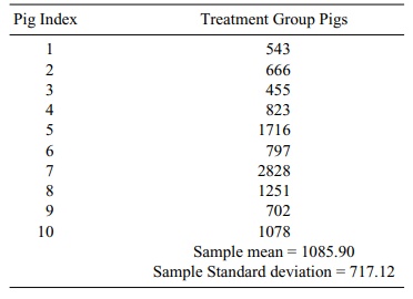Suppose we have a random sample of size 10. Consider the pig blood loss data (treatment group) shown in Table 8.2, which reproduces the treatment data from Table 8.1.

TABLE 8.2. Pig Blood Loss Data (ml)

Let us use the method in Section 8.4 based on the t statistic to generate a para-metric 95% confidence interval for the mean. Then we will show you how to gener-ate a bootstrap percentile method confidence interval based on just 20 bootstrap samples. We will then show you a better approximation based on 10,000 bootstrap samples. The result based on 10,000 bootstrap samples requires intensive comput-ing, which we do using the software package Resampling Stats.

Recall that the parametric confidence interval based on t is [ – C(S/√n), X + C(S/√n)], where S is the sample standard deviation,  is the sample mean, and C is the constant taken from the t distribution with n – 1 degrees of freedom, where n is the sample size and C satisfies the relationship P(–C ≤ t ≤ C) = 0.95. In this case, n = 10 and df = n – 1 = 9. From the table of Student’s t we see that C = 2.2622.

Now, in our example,  = 1085.90 ml and s = 717.12 ml. So the confidence in-terval is [1085.9 – 2.2622(717.12/√10, 1085.9 + 2.2622(717.12/√10] = [1085.9 – 513.01, 1085.9 + 513.01] = [572.89, 1598.91]. Similarly, for a 90% interval the val-ue for C is 1.8331; hence, the 90% interval is [1085.9 – 415.7, 1085.9 + 415.7] = [670.2, 1501.6].

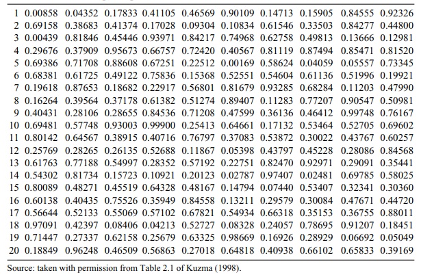
Now let us generate 20 bootstrap samples of size 10 and calculate the mean of each bootstrap sample. We first list the samples based on their pig index and then we will compute the bootstrap sample values and estimates. To generate 20 boot-strap samples of size 10 we need 200 uniform random numbers. The following 10 × 20 table (Table 8.3) provides the 200 uniform random numbers. Each row repre-sents a bootstrap sample. The pig indices are obtained as follows:

If the uniform random number U is in [0.0, 0.1), the pig index I is 1.

If the uniform random number U is in [0.1, 0.2), the pig index I is 2.

If the uniform random number U is in [0.2, 0.3), the pig index I is 3.

If the uniform random number U is in [0.3, 0.4), the pig index I is 4.

If the uniform random number U is in [0.4, 0.5), the pig index I is 5.

If the uniform random number U is in [0.5, 0.6), the pig index I is 6.

If the uniform random number U is in [0.6, 0.7), the pig index I is 7.

If the uniform random number U is in [0.7, 0.8), the pig index I is 8.

If the uniform random number U is in [0.8, 0.9), the pig index I is 9.

If the uniform random number U is in [0.9, 1.0), the pig index I is 10.

TABLE 8.3. Bootstrap Sample Uniform Random Numbers

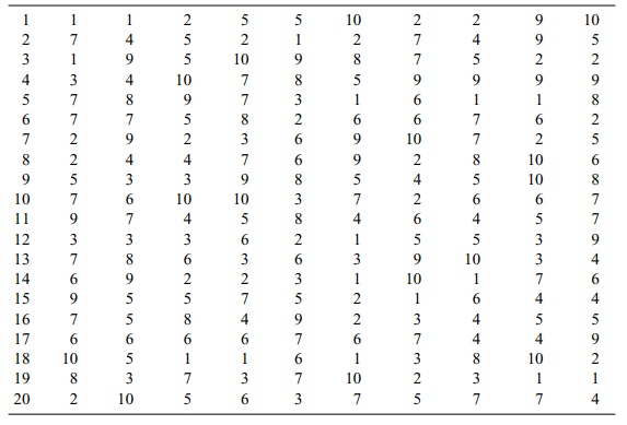
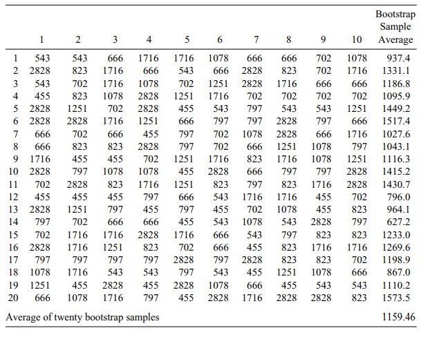
In Table 8.4, the indices replace the random numbers from Table 8.3. Then in Table 8.5, the treatment group values from Table 8.2 replace the indices. The rows in Table 8.5 show the bootstrap sample averages with the bottom row showing the av-erage of the 20 bootstrap samples.

Note in Table 8.5 the similarity of the overall bootstrap estimates to the sample estimates. For the original sample the sample, mean was 1085.9 and the estimate of its standard error was 226.77. By comparison, the bootstrap estimate of the mean is 1159.46 and its bootstrap estimated standard error is 251.25. The standard error is obtained by computing a sample standard deviation for the 20 bootstrap sample es-timates in Table 8.4.

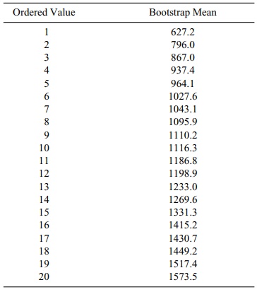
Bootstrap percentile confidence intervals are obtained by ordering the bootstrap estimates from smallest to largest. For an approximate 90% confidence interval, the 5th percentile and the 95th percentile are taken as the endpoints of the interval.

TABLE 8.4. Random Pig Indices Based on Table 8.3

Because there are 20 estimates, the interval is from the second smallest to the next to largest, as 5% of the observations are below the second smallest (1/20) and 5% are above the second largest (1/20). Consequently, the 90% bootstrap percentile method confidence interval for the mean is obtained by inspecting Table 8.6, which orders the bootstrap mean estimates.

Since observation number 2 in increasing rank order is 796.0 and observation 19 in rank order is 1517.4, the confidence interval is [796.0, 1517.4]. Compare this to the parametric 90% interval of [670.2, 1501.6]. This difference between the two calculations could be due to the nonnormality of the data.

We will revisit the results for a random sample of 200 after computing the more precise estimates based on 10,000 bootstrap samples. Using 10,000 bootstrap sam-ples, we will also be able to compute and compare the 95% confidence intervals. These procedures will require the use of the computer program Resampling Stats.

Resampling Stats is a product of the company of the same name founded by Ju-lian Simon and Peter Bruce to provide software tools to teach and perform statisti-cal calculations by bootstrap and other resampling methods. Their software is dis-cussed further in Chapter 16.

Using the Resampling Stats software, we created the following program (dis-played in italics) in the Resampling Stats language:

data (543 666 455 823 1716 797 2828 1251 702 1078) bdloss

maximize z 15000

mean bdloss mb

stdev bdloss sigb

TABLE 8.5. Bootstrap Sample Blood Loss Values and Averages Based on Pig Indices from Table 8.4

print mb sigb

repeat 10000

sample 10 bdloss bootb

mean bootb mbs$

stdev bootb sigbs$

score mbs$ z

end

histogram z

percentile z (2.5 97.5) k

print mb k

The first line of the code is the data statement. An array is a collection or vector of values stored under a common name and indexed from 1 to n, where n is the ar-ray size. It takes the 10 blood loss values for the pigs and stores it in an array called bdloss; bdloss is an array of size n = 10.

TABLE 8.6. Bootstrap Estimates of Mean Blood Loss in Increasing Order

The next line is the maxsize statement. This statement specifies an array size of 15,000 for the array z. By default, arrays are normally limited to be 1000 in length. So the n = 15,000 for the array z. We will be able to generate up to 15,000 bootstrap samples (i.e., B = 10,000 for the number of bootstrap samples in this application, but the number could have been as large as 15,000).

The next two statements, mean and stdev, compute the sample mean and sample standard deviation, respectively, for the data in the bdloss array. The results are stored in the variables mb and sigb for the mean and standard deviation, respective-ly. The print statement tells the computer to print out the results.

The repeat statement then tells the computer how many times to repeat the next several statements. It starts a loop (like a do loop in Fortran). The sample statement tells the computer how to generate the bootstrap samples. The number 10 tells it to sample with replacement 10 times.

The array bdloss appears in the position to tell the computer to sample from the data in the bdloss array. Then the name bootb is the array to store the bootstrap sam-ple. The next two statements produce the sample means and standard deviations for the bootstrap samples. The score statement tells the computer to keep the results for the means in a vector called z. The end statement indicates the end of the loop that does the calculations for each of the 10,000 bootstrap samples.

The histogram statement then takes the results in z and creates a histogram, auto-matically choosing the number of bins (i.e., intervals for the histogram), the bin width and the center of each bin. The percentile statement tells the computer to list the specified set of percentiles from the distribution determined by the array of bootstrap means that are stored in z (like the last column in Table 8.5 from the sam-ple of 20 bootstrap estimates of mean blood loss).

When we choose 2.5 and 97.5, these values will represent the endpoint of a boot-strap percentile method confidence interval at the 95% confidence level for the mean based on 10,000 bootstrap samples. The final print statement prints the sam-ple mean of the original sample and the endpoints of the bootstrap confidence inter-val. In real time, the program took 1.5 seconds to execute; the results (in bold face) appeared exactly as follows:

MB = 1085.9

SIGB = 717.12

Vector no. 1: Z

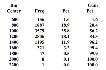
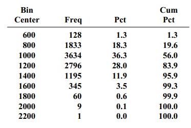
Note: Each bin covers all values within 100 of its center.

MB = 1085.9

K = 727.1   1558.9

Interpreting the output, MB represents the sample mean for the original data and SIGB the standard deviation for the original data. The histogram is for Vector no. 1, the array Z of bootstrap sample means. K is an array of size n = 2 with its first el-ement the 2.5 percentile from the histogram of bootstrap means and the second ele-ment the 97.5 percentile from that histogram.

Using 10,000 random samples, the bootstrap percentile method 95% confidence interval is [727.1, 1558.9]. Notice that this is much different from the confidence interval we obtained by assuming a normal distribution. Recall that that interval was [572.89, 1598.91], which is much wider than the interval produced by the boot-strap percentile method. This result is due to the fact that the distribution for the individual observations is not normal and the sample size of 10 is too small for the central limit theorem to apply to the sample mean.

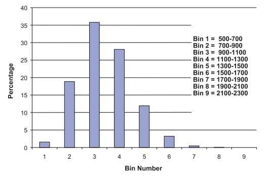
Figure 8.3. Histogram of bootstrap means for the pig treatment group blood loss used for 95% bootstrap percentile method confidence interval.

Not only does the bootstrap give a tighter interval than the normal approxima-tion, but also the resulting interval is more realistic based on the sample we ob-served! Figure 8.3 shows the bootstrap histogram that indicates a skewed distribu-tion for the sampling distribution of the mean.

To obtain a 90% bootstrap confidence interval using Resampling Stats, we need only change the percentile statement above to the following:

percentile z (5.0 95.0) k

The resulting interval is [727.1, 1558.9]. Recall that, based on only 20 bootstrap samples, we found [796.0, 1517.4] and from normal distribution theory [670.2, 1501.6]. Again, the two bootstrap results are not only different from the results ob-tained by using the normal distribution, but also are more realistic. We see that 20 samples do not yield an adequate bootstrap interval estimate.

There is a large difference between 20 bootstrap samples and 10,000 bootstrap samples. The histogram from the Monte Carlo approximation provides a good ap-proximation to the bootstrap distribution only as the number of Monte Carlo itera-tions (B) becomes large. For B as high as 10,000, this distribution and the resulting confidence interval will not change much if we continue to increase B.

However, when B is only 20 this result will not be the case. We chose a small value of 20 for B so that we could demonstrate all the steps of the bootstrap interval estimate without having to resort to the computer. But to produce an accurate interval, we did need a large B and resorted to the Resampling Stats program.

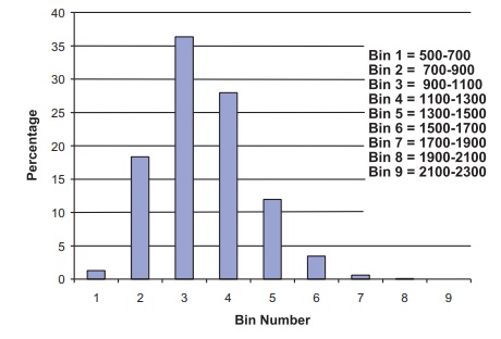
Figure 8.4. Second histogram of bootstrap means for the pig treatment group blood loss. Used for 90% bootstrap percentile method confidence interval.

Subsequently, we found an estimate for the 90% bootstrap confidence interval by using a different set of 10,000 bootstrap samples; hence, the histogram (refer to Figure 8.4) is slightly different from that produced for the 95% confidence interval. The results for this Monte Carlo approximation are as follows (shown in bold face type):

MB = 1085.9

SIGB = 717.12

Vector no. 1: Z

Note: Each bin covers all values within 100 of its center.